潜空间扩散与 Stable Diffusion 架构

所属方向：生成范式 ｜ 难度：进阶 ｜ 前置知识：VAE 结构与 0.18215、DDPM 训练目标与采样流程（$\bar\alpha_t$、$\varepsilon$ 预测器、DDIM 那一步怎么走都在那两篇推过，这里直接用结论）
关键词：潜空间扩散、LDM、Stable Diffusion、UNet、交叉注意力、scale factor

01. 为什么需要它

潜空间扩散的主要收益是降低生成网络处理的空间位置数。下面把一个 SD1.5 风格 UNet 原样放大到像素空间做静态对照；这不是所有像素扩散的成本，也不是实际 GPU 显存或延迟测试。

账本依据 SD1.5 的配置和 diffusers 构造逻辑（附录 unet_ledger.py）。有个历史命名陷阱：attention_head_dim=8 在该模型的构造逻辑中实际表示 8 个头，不是每头 8 维；320 通道对应每头 40 维。修正头数、真实 skip 通道和 Transformer 外层投影后，账本参数量为 859,520,964，与文中参照值 859,522,604 差 1,640（约 0.00019%）。这是静态近似，不能把参数接近当成峰值显存验证。若朴素实现显式保存注意力矩阵，512² 像素上的首层需要

$$512^2\times512^2\times8\times2\ \text{bytes}=2^{40}\ \text{bytes}=1\ \text{TiB}$$

这里按二进制单位计算为 1 TiB；同层 64² latent 需要 256 MiB，矩阵元素数相差 4096 倍。SDPA / FlashAttention 可以不保存完整矩阵，所以这些是朴素物化成本，不是现代实现的必然显存占用。

把像素模型 attention 只放最深层，静态账本得到单步约 $1.4455\times10^{13}$ MAC；latent 版本约 $4.0164\times10^{11}$ MAC，相差 36.0 倍。对应逐层激活累计约 12.94 GiB 与 2.04 GiB，尚未模拟张量生命周期、重计算、优化器或融合内核。VAE 编解码是额外开销，占比随采样步数、分辨率和实现改变，本实验没有测量它。

压缩也引入信息取舍。latent_lab.py 用一张样例图做块 DCT，只保留 192 个系数中的 4 个，得到 94.91% 能量和约 22.06 dB PSNR。能量不是语义信息量，高频中的文字笔画、边缘、细小物体仍可能很重要；该单图线性实验不能证明 VAE 只删除“人眼不关心”的内容。

实际 LDM 用学习到的感知压缩来减小扩散的工作空间，并同时权衡重建质量、生成质量和成本。像素扩散、级联超分也能实现高分辨率生成，潜空间是有用路线而非唯一可行路线。

02. 最小可用理解

三句话：

1. 机制：先训一个 VAE 把图像 $x$ 压成潜特征 $z=\mathcal{E}(x)$（f=8 下采样、3 通道变 4 通道，512×512×3 变 64×64×4，压缩率 48 倍），然后把 DDPM 原封不动地搬到 $z$ 上做，条件（文本）通过交叉注意力在 UNet 内部注入。
2. 成本：卷积部分的算力正比于空间 token 数，所以正好除以 $f^2=64$；但 self-attention 是 $O(N^2)$，压缩后从「根本放不下」变成「贵但可做」。实测 512px 下像素空间与潜空间的单步 MAC 比 678.6 倍，只看卷积部分是 64.0 倍。
3. 效果与代价：扩散模型不再直接对像素负责，可还原的细节受 VAE 限制——VAE 解不回来的细节，扩散模型画得再好也出不来。这是潜空间模型的一项误差来源，不能单独解释文字或手指等全部生成错误。

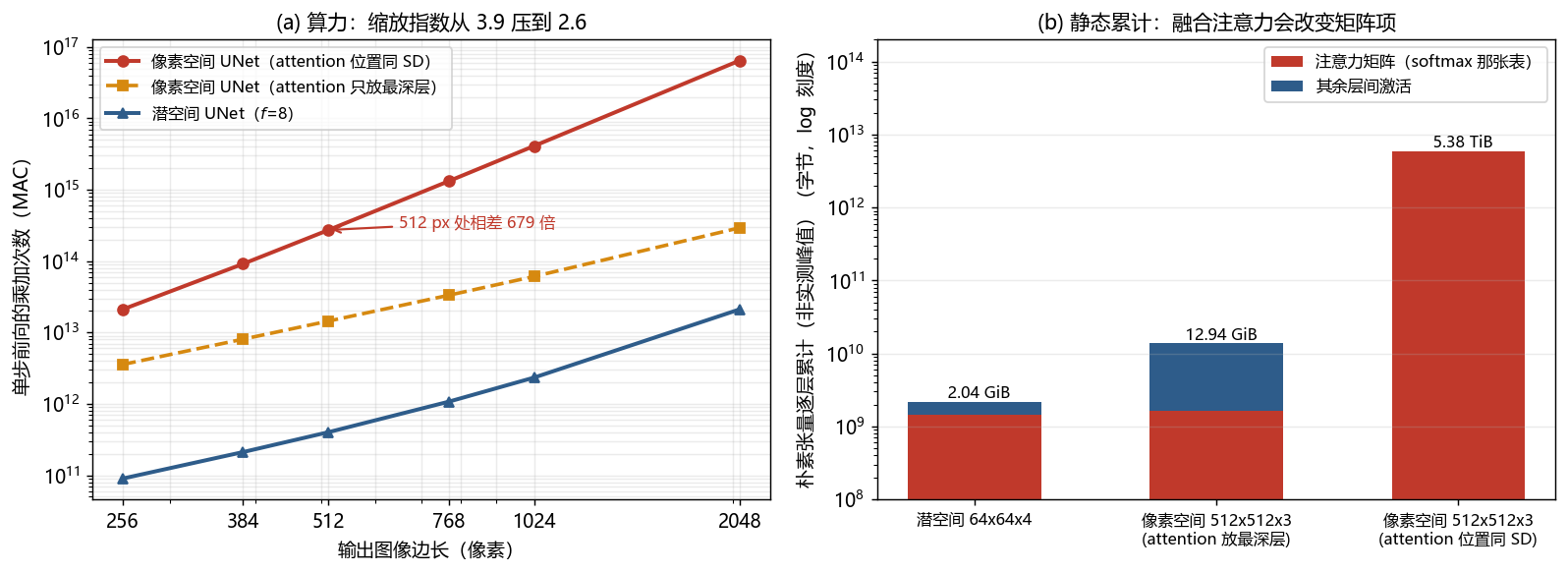
这张图看静态 MAC 随边长变化的趋势：在本扫描区间，像素同拓扑约为边长的 3.87 次方，latent 约为 2.61 次方。512px 处约相差 679 倍。右图是朴素实现的逐层张量累计，不是实测峰值；使用融合注意力时，红色矩阵项会显著改变。

03. 数学推导

3.1 两阶段目标

LDM 是两阶段训练，不是给同一个联合损失设置一个任意 λ：

$$\text{阶段一：}\min_{\phi,\psi}L_{\text{AE}}(\phi,\psi),\qquad\text{阶段二：固定 }(\phi,\psi)\text{ 后 }\min_\theta L_{\text{LDM}}(\theta)$$

第一阶段优化自编码器的重建、正则与感知/对抗目标；第二阶段冻结编码器与解码器，只优化 latent 扩散目标。这样扩散训练所见的 latent 分布保持固定。联合训练是另一类研究方案，需要额外处理两侧变化。

3.2 感知压缩：压缩率从哪来

VAE 的编码器把 $x\in\mathbb{R}^{H\times W\times 3}$ 映到 $z\in\mathbb{R}^{h\times w\times C}$，其中 $h=H/f$、$w=W/f$。定义压缩率

$$r=\frac{3\,f^{2}}{C}$$

$f$ 是空间下采样倍数，$C$ 是潜通道数。SD 用 $f=8$、$C=4$，所以 $r=48$。这个式子值得停一下：$f$ 和 $C$ 是两个独立的旋钮，$f$ 控制空间上省多少（直接决定 UNet 卷积部分省多少，因为卷积算力正比 $h\times w$），$C$ 控制每个位置带多少信息。附录表 [A] 里扫了这两个旋钮的交叉组合：$f=8,C=4$ 时线性重建只有 22.06 dB，把 $C$ 从 4 提到 16 能到 27.56 dB，把 $f$ 从 8 降到 4 也能到 26.09 dB——两条路都能换质量，但 $f$ 的每一档都同时把算力除以 4，而 $C$ 只影响通道数。LDM 论文选 $f=8$ 就是在这条帕累托前沿上取的点。

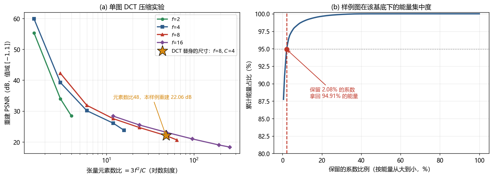
图中星号只是与 SD 相同张量尺寸的 DCT 教学替身，不是实测 SD VAE 的 PSNR。不同曲线来自同一张图的不同块大小与保留系数数目；右侧能量比例依赖图像和基底，不代表感知信息保留率。

感知压缩通常结合像素重建、LPIPS 和对抗目标。逐像素 L2 在重建不确定时倾向条件均值，可能使细节变模糊；感知项约束特征而非逐像素对应。但 L2 不会因为“高频系数数量多”就被低能量项支配：正交变换下 Parseval 等式保持总平方误差。是否使用某项应看具体配方与消融。

3.3 潜空间扩散目标

VAE 冻结之后，扩散这一半就是把 DDPM 的每个符号里的 $x$ 换成 $z$。前向过程：

$$z_t=\sqrt{\bar\alpha_t}\,z_0+\sqrt{1-\bar\alpha_t}\,\varepsilon,\qquad \varepsilon\sim\mathcal{N}(0,1)$$

训练目标是噪声预测，条件 $c$（文本的 CLIP 编码）只通过 UNet 内部的交叉注意力进入：

$$L_{\text{LDM}}=\mathbb{E}_{z_0,\,\varepsilon,\,t}\Big[\big\|\varepsilon-\varepsilon_\theta(z_t,t,c)\big\|_2^2\Big]$$

注意这个目标和像素空间的形式一字不差——这正是「搬进潜空间」这个动作的全部：不是发明新模型，是换了个更小的工作空间。上一篇文章讲的 CFG、上上篇讲的 DDIM 采样器，在这里原样成立。

3.4 scale factor：为什么必须有

扩散训练需要固定 latent 的尺度约定。单位数据方差时，SNR 是 $\bar\alpha_t/(1-\bar\alpha_t)$，不是 $\bar\alpha_t$ 本身。SD1.x 常用乘数 $s=0.18215$，对应原始标准差约 5.49、方差约 30.14；编码后要乘 s，解码前除 s。

把 $z$ 整体乘 $k$ 倍，信噪比就乘 $k^2$：

$$\mathrm{SNR}_{\text{eff}}(t)=\frac{\bar\alpha_t\,(k\sigma_z)^2}{1-\bar\alpha_t}$$

也就是说，网络在时间步 $t$ 实际体验到的难度，等于调度表里另一个时间步 $t'$ 的难度。附录脚本 [B2] 把这个对应关系算了出来（cosine 调度、$T=1000$、参考 $t=500$）：scale 错 2 倍，等效于把 t=500 映射到约 t′=292.7（差 −207.3 步）；错 4 倍是 −348.9 步；错 0.5 倍是 +205.7 步。这是参考时刻的等效 SNR 变化，不是固定的全局时间平移。

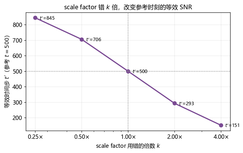
这张图在固定参考 t=500 上比较尺度倍数 k 与等效时间 t′，曲线经过 k=1、t′=500。这种映射是非线性的，不是把整条时间表平移固定步数；−207.3 只是本调度在这个参考时刻、k=2 的差值。

还有一层：全局缩放只解决「整体方差」的问题，解决不了「通道之间」。附录 [B] 用样例照片的 DCT 特征实测（不是 VAE 权重输出）：8 个通道的标准差从 8.0681 一直掉到 0.5386，相差 14.98 倍。对线性-高斯去噪器，第 $j$ 个通道的不可约残差是

$$\mathrm{MSE}_j(t)=\frac{\bar\alpha_t\,\sigma_j^2}{\bar\alpha_t\,\sigma_j^2+1-\bar\alpha_t}$$

这里是预测 ε 时的 Bayes 最小 MSE，按通道相加得到最小期望损失；它不是参数梯度份额。toy DCT 通道在 $\bar\alpha=0.1$ 时最高方差通道占约 51.28% 的该残差，说明全局缩放不消除通道尺度差异，但不能据此解释真实 SD 的细节质量，本文没有测量真实 VAE latent。

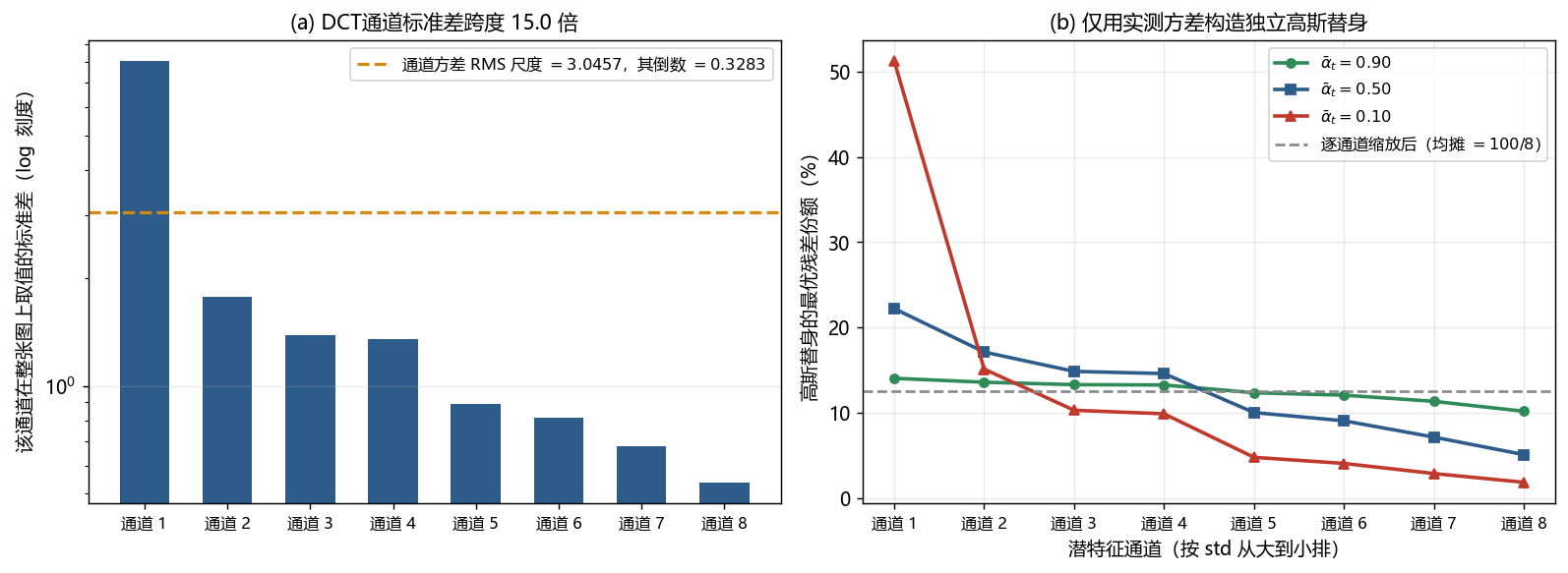
这张图要看什么：左图是 8 个通道各自的 std（对数刻度），橙色虚线是通道方差均值的平方根（3.0457，不含通道均值之间的差异）——它的倒数 0.3283 就是 SD 那个 0.18215 的类比物，注意全局缩放之后通道之间的 15 倍跨度原封不动。右图是三条 $\bar\alpha_t$ 下各通道分到的 loss 份额：三条曲线都从左往右掉，灰色虚线是「逐通道缩放后」的均摊线 12.5%。$\bar\alpha_t$ 越小（噪声越大），失衡越严重。

3.5 交叉注意力：条件怎么进来

文本 $y$ 先过 CLIP 文本编码器得到 $\tau_\theta(y)\in\mathbb{R}^{77\times 768}$，然后进 UNet 内部的 Transformer 块。每个 Transformer 块有两个注意力，分工不同：

$$\mathrm{attn}_1=\mathrm{softmax}\Big(\frac{QK^\top}{\sqrt d}\Big)V,\quad Q,K,V\ \text{都来自图像 token}\qquad\qquad\mathrm{attn}_2=\mathrm{softmax}\Big(\frac{QK^\top}{\sqrt d}\Big)V,\quad Q\ \text{来自图像 token},\ K,V\ \text{来自文本}$$

$\mathrm{attn}_1$ 是 self-attention，管图像内部的空间关系；$\mathrm{attn}_2$ 是 cross-attention，管「这段话在这个位置要什么」。关键在成本结构：图像 token 数 $N=h\times w$，文本 token 数固定 $T=77$，所以

$$\mathrm{attn}_1\ \text{的注意力矩阵是}\ N\times N,\qquad \mathrm{attn}_2\ \text{的是}\ N\times 77$$

对 token 数 N，self-attention 的矩阵计算二次增长，cross-attention 在固定文本长度下近似线性增长。修正账本后，cross-attention 的 MAC 占比从 64² latent 的 4.00% 降到 256² 的 1.11%；绝对 MAC 仍从约 $1.60\times10^{10}$ 升到 $2.35\times10^{11}$，占比下降不能说它“不涨钱”。

单头注意力输出 $AV$ 满足 $\mathrm{rank}(AV)\le\min(T,d_{\text{head}})$，这里 T=77。附录单头、d=320 的随机矩阵实验得到秩 77。真实 SD 是多头：各头拼接后秩上界可达 $\min(C,H_{\text{heads}}T)$，再加残差、非线性与多层处理，不能声称整个 UNet 只有 77 个自由度。文本与细粒度空间控制仍是不同接口，但这个单头秩实验不能单独证明 ControlNet 的必要性。

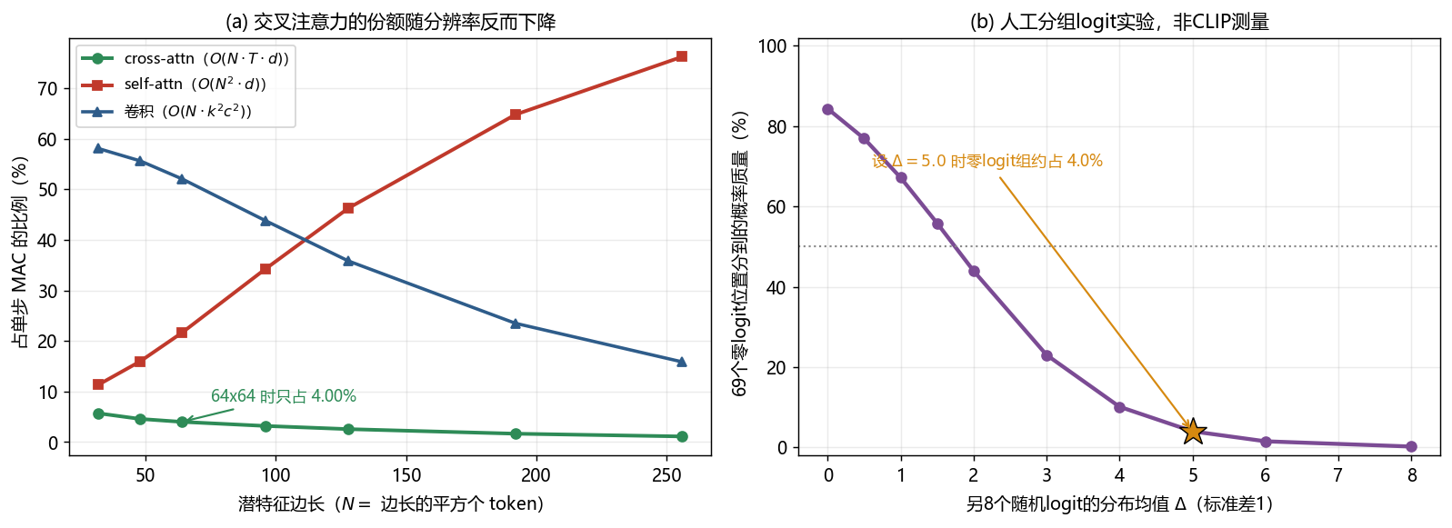
左图是修正后的静态 MAC 占比。右图只是人为设定的“许多等 logit 位置”在 softmax 中累加概率质量的示意：真实 CLIP 即使使用相同 padding token ID，各位置经过位置编码与上下文注意力后的向量也不相同，不能把它们当成一个相同 EOS embedding 集团。是否传 mask 应核对具体 pipeline。

04. 代码实现

三段最小实现，全部 numpy，/usr/local/bin/python3（3.10.5）直接可跑；完整脚本在文末附录。

4.1 块正交编码器（VAE 的替身）

没有 torch 和真实权重，我用一个线性正交编码器当 VAE 的替身：切成 $f\times f\times 3$ 的块、做三维可分离 DCT、只留能量最大的 $C$ 个系数。它与该 VAE 的张量形状及元素压缩率对应——潜特征形状就是 $(h, w, C)$，压缩率就是 $\frac{3f^2}{C}$，变量名和 3.2 节的符号一一对应。用它做替身的好处是把「压缩率」这一个变量单独隔离出来了。

def block_basis(f):
    """f x f x 3 块的可分离正交基，展平顺序 (channel, row, col)。"""
    df = dct_matrix(f)
    return np.kron(dct_matrix(3), np.kron(df, df))

def encode_decode(img, f, c_keep):
    """img: [H, W, 3]，值域 [-1, 1]。返回潜特征、重建图、能量占比。"""
    h, w, _ = img.shape
    patches = to_blocks(img, f)                  # [h*w/f^2, 3*f*f]
    b = block_basis(f)
    coef = patches @ b.T                         # 正交变换，能量不变
    energy = np.mean(coef ** 2, axis=0)          # 每个基函数的平均能量
    keep = np.sort(np.argsort(energy)[::-1][:c_keep])
    latent = coef[:, keep].reshape(h // f, w // f, c_keep)
    rec = from_blocks(coef[:, keep] @ b[keep, :], h, w, f)
    frac = float(energy[keep].sum() / energy.sum())
    return latent, np.clip(rec, -1.0, 1.0), frac

真实输出（一张 512×512 照片）：

encode_decode(img, 8, 4)
  latent.shape = (64, 64, 4)      # 与 SD 的潜特征形状完全一致
  压缩率     = 48.0x              # 3*8^2/4
  PSNR       = 22.06 dB           # 线性重建的上限就在这附近
  保留能量   = 94.9081%           # 扔掉的 98% 系数只占 5.09% 的能量

22.06 dB 是这一张图在该 DCT 选择和裁剪策略下的结果，不是所有线性编码器的上限，也不是 SD VAE 的重建质量。真实非线性编码器可能学到不同的特征表示；没有跑权重就不能量化它比这个替身好多少。

4.2 UNet 账本（参数量对拍）

记账模型按 SD 1.5 的拓扑走一遍：4 个分辨率、每层 2 个 ResNet（上采样路径 3 个）、attention 放在下采样路径的第 0/1/2 层和上采样路径对应的层、中段是 ResNet-Transformer-ResNet。

def resnet(self, res, cin, cout):
    """ResnetBlock2D：GroupNorm-Conv-GroupNorm-Conv + timestep 注入 + shortcut。"""
    n = res * res
    self.group_norm(n, cin)
    self.conv2d(3, cin, cout, res, res)
    self.group_norm(n, cout)
    self.conv2d(3, cout, cout, res, res)
    self.linear(1, TEMB_CH, cout)        # time_emb_proj: [1280] -> [cout]
    if cin != cout:
        self.conv2d(1, cin, cout, res, res)   # conv_shortcut（上采样路径必带）

def transformer_block(self, res, ch, ctx_len):
    """self-attn -> cross-attn -> FFN（GEGLU，4 倍扩张）。"""
    n = res * res
    heads = NUM_HEADS
    ...  # Q/K/V 投影 + 两次注意力 + GEGLU

真实输出：

build_unet(64, 64, 4, 4)      # 潜空间
  params = 859,520,964        # 官方 SD 1.5 UNet = 859,522,604，差 1,640（约 -0.00019%）
  MAC    = 4.0164e+11
  构成   = conv 52.1%  self_attn 21.6%  cross_attn 4.0%  ffn 19.1%  proj 3.2%
build_unet(512, 512, 3, 3)    # 同一拓扑搬回像素空间
  MAC    = 2.7256e+14         # 是潜空间的 678.6 倍

账本中 FFN 占约 19.1% MAC、cross-attention 约 4.0%，需要同时考虑投影、卷积和注意力矩阵乘。上采样 ResNet 拼接当前特征与 skip，其通道数是两者相加，跨层时并不总等于输出通道的两倍；修正版按 skip 栈逐项消费。

4.3 交叉注意力（10 行，含秩的验证）

def cross_attn_demo(rng, d=320, side=64, ctx_len=77):
    n_img = side * side
    q = rng.standard_normal((n_img, d)) / np.sqrt(d)      # 图像 token
    k_txt = rng.standard_normal((ctx_len, d)) / np.sqrt(d)  # 文本 token
    v_txt = rng.standard_normal((ctx_len, d)) / np.sqrt(d)
    a = softmax((q @ k_txt.T) / np.sqrt(d), axis=-1)      # [4096, 77]
    out = a @ v_txt                                        # [4096, 320]
    rank = int(np.sum(np.linalg.svd(out, compute_uv=False)
                      > np.linalg.svd(out, compute_uv=False)[0] * 1e-8))
    print(a.shape, out.shape, rank)

真实输出：

(4096, 77) (4096, 320) 77

这个单头教学例子的秩为 77，验证的是单次矩阵乘积的秩界。多头、残差与深层非线性不受同一个“77 维全局瓶颈”约束。

05. 工业级实现对照

对照 diffusers 的 UNet2DConditionModel（huggingface/diffusers · unet_2d_condition.py，symbol UNet2DConditionModel.forward；以 2026-09 时的实现为准，上游会重构）：

时间步通过 ResBlock 注入。 SD1.5 常见实现把时间 embedding 投影后加到特征上；原始 DDPM 实现也有加性注入，不能说原版 DDPM 使用 AdaGN、到 SD 才改成加法。scale-shift norm 等方式属于其他配置选择，比较时应指出具体模型。

SD1.5 的文本通常通过 cross-attention 注入。 通用 UNet2DConditionModel 还支持 class embedding、附加条件以及 only_cross_attention 等配置，不能把 SD1.5 的一条路径说成这个类的永恒约束。SDXL 还有 pooled 文本、尺寸和裁剪条件；SD2.x 并不是这里所有额外条件接口的来源。

attention 后端影响实际显存。 UNet 构造实现 为历史兼容设置 num_attention_heads = num_attention_heads or attention_head_dim，SD1.5 因而是 8 头。64² latent 的单层显式矩阵约 256 MiB；SDPA / FlashAttention 可避免完整物化，是否使用取决于设备、版本和配置。

scale factor 放在 VAE 的配置里，不在 UNet 里。 AutoencoderKL 的 config 带 scaling_factor: 0.18215，pipeline 在 vae.encode(...).latent_dist.sample() 之后乘上它、在 vae.decode 之前除回来。UNet 见到的是训练约定缩放后的潜特征。换 VAE（比如 SD 2.x 或 SDXL 的 VAE）要连 scaling_factor 一起换，见 3.4 节的等效时间映射。

64² latent 的中段在 8²。 三次下采样后到达 8²；skip 栈包含 conv_in、每个 ResNet/attention 组合的输出与下采样输出，attention 不是在同一 ResNet 之外额外再存一条独立 skip。上采样块依次消费这些特征，所以输入通道必须逐项记账。

06. 代价与边界

代价一：解码器与瓶颈限制重建和生成。 被编码过程丢掉的信息无法保证按原样还原，固定解码器也限制可生成的图像集合。但手指、文字错误还可能来自生成模型和数据，不能把一类生成错误全部归因于 VAE。输入重建误差也不是生成样本误差的严格上限。

代价二：尺度约定要成对维护。 toy 的通道跨度说明一个全局标量不能独立归一化每个通道。真实 VAE 是否需要逐通道处理必须测量；使用预训练扩散模型时还要保持它训练时的 latent 语义和配置，不能只改系数。

代价三：文本不直接指定每个空间位置。 更精确的姿态、深度、边缘控制常加入空间条件分支，但原因涉及任务表示与训练，不是整个 UNet 输出秩只能为 77。多头注意力的秩上界见 3.5 节。

选择时看保真需求与实测成本。 严格像素保真的编辑、文档和重建任务需要评估 VAE 引入的误差，可能选择更低压缩、多尺度或像素方案。超高分辨率并不自动排除 latent 模型：分块、融合注意力、不同生成骨干都会改变成本。本文 2048px 对照的朴素逐层累计约 352.53 GiB，既不是实测峰值，也不是 SDXL 的数字。

07. 经典论文脉络

• Taming Transformers（VQGAN, 2012.09841）：先把「感知压缩 + 在压缩空间里做生成」这条路走通，但它用的是离散 token + 自回归 Transformer。LDM 的感知压缩部分直接继承自它。
• DDPM（2006.11239）：确立像素空间扩散的训练目标和采样流程，是 LDM 搬进潜空间之前的那块地基（前置篇已推）。
• LDM / Stable Diffusion（2112.10752）：本文锚点。两个贡献——连续 VAE 潜空间 + 交叉注意力条件注入；前者解决算力，后者把「无条件/有条件」的分支统一成一个可外推的接口（CFG 的舞台）。
• Imagen（Saharia et al., 2022；2205.11487）：反方意见。证明像素空间级联扩散（64→256→1024 逐级超分）+ 更强的文本编码器也能达到顶尖质量，说明潜空间不是唯一解；它给出的重要观察是「文本编码器的重要性高于 UNet 规模」。
• SDXL（2307.01952）：潜空间路线的工程演进——更大 UNet、双文本编码器、多宽高比分桶和额外尺寸条件。

一句话串起来：VQGAN 证明了压缩空间里能生成，DDPM 证明了扩散能生成，LDM 把两者拼起来并解决了条件注入，Imagen 提出反例，SDXL 证明了这条路线的上限还没到。

08. 常见误解

「潜空间扩散等价于像素扩散加一个 VAE。」 VAE 改变了数据表示、尺度与可还原的信息，训练好的两个去噪器不能无成本互换；差异不能简单归结为“高频全部被删掉”。

「保留 95% 能量就等于保留 95% 信息。」 能量是特定数值空间的平方和，不是感知信息量；小字等低能量结构可能极为重要。本文单图 DCT 只展示能量集中性，真实 VAE 必须另做重建与感知评估。

「0.18215 是个可以随便调的超参。」 它是 $1/\sigma_z$，是潜空间统计量的倒数。错 2 倍等于在本文参考 t=500 处映射到约早 207 步的等效 SNR（3.4 节实测），调度表两头本来分工明确的步数预算全被挪用。换 VAE 必须连它一起换，不存在「微调一下」。

「交叉注意力很贵，所以推理慢。」 实测它只占单步 MAC 的 4.00%（64×64 潜特征），分辨率越高占比越低。真正贵的是 self-attention（21.6%）和卷积（52.1%）。把推理优化火力对准 cross-attention 大方向就错了。

「SD 的 UNet 只需按通道翻倍估一下。」 跨层 skip、Transformer 外层投影、不同 attention 配置都会影响账本。尤其 SD1.x 配置中的 attention_head_dim=8 是历史头数命名，不能据此算成 40 个头。

09. 动手验证

两份脚本都在附录，unet_ledger.py 仅用标准库，latent_lab.py 需要 numpy 与 Pillow，并需要通过 --image 提供图片或在仓库中使用默认样例（不需要 torch）：

python unet_ledger.py --sweep
python latent_lab.py

我实跑的关键输出，你可以对：

unet_ledger.py
  潜空间 params = 859,520,964（官方 859,522,604，差 1,640（约 -0.00019%））
  潜空间单步 MAC = 4.0164e+11；像素空间 = 2.7256e+14，678.6 倍
  只看卷积部分 = 64.0 倍（正好是 f^2）
  cross-attn 占比：64x64 4.00% -> 256x256 1.11%
  分辨率扫描加速比：256px 234.3x，512px 678.6x，1024px 1754.7x

latent_lab.py
  f=8, C=4：PSNR 22.06 dB，保留能量 94.9081%
  能量最大的 1% 系数（2 个）携带 91.01% 的总能量
  8 个通道 std 相差 14.98 倍；alpha_bar=0.1 时 top1 通道占 51.28% 的 loss
  scale 错 2 倍 -> 等效时间步偏移 -207.3 步
  cross-attn 输出的秩 = 77（self-attn 对照 = 320）
  padding 组在内容优势为 0 时抢走 84.38% 的注意力质量

两个练习：把 --image 换成自己的图，比较 DCT 能量集中度与重建质量；把 NUM_HEADS 从 8 改为 4，在通道宽度不变时，注意力矩阵存储减半，而 QK/AV 的总 MAC 基本不变。该配置实验演示公式，不代表修改预训练模型后可直接使用。

10. 延伸阅读

按知识树的依赖链走：

• DDPM 训练目标与采样流程：本文 3.3 节那行目标的完整推导。
• VAE 结构与 0.18215：VAE 一侧的全部细节，包括那个数字的来历。
• 分类器无关引导 CFG 的代价与调法：cross-attention 这条条件通路在采样时怎么被外推。
• 从 DDIM 到高阶采样器：潜空间里怎么把 1000 步压到 20 步。
• FlashAttention 为什么不需要存下注意力矩阵：图 1b 那根红柱子怎么消掉。
• 已发布相邻节点：DiT（Transformer 生成骨干，具体条件方式依模型而异）、流匹配（另一种连续生成路径）。VQ-VAE 与 VQGAN 的专题仍待补齐。

附录：完整代码

09 节用到的脚本全文如下（unet_ledger.py、latent_lab.py、make_figures.py）。复制到本地存成同名文件，按各脚本开头的依赖说明准备环境后即可运行。

unet_ledger.py

#!/usr/bin/env python3
# -*- coding: utf-8 -*-
"""SD 系 UNet 的算力 / 显存账本：像素空间 vs 潜空间。

这个脚本不跑真正的卷积（环境里没有 torch），而是按 SD 1.5
UNet2DConditionModel 的公开配置把每一层的形状、参数量、MAC 数、需要保存的
激活字节数逐一累加出来。数字是静态算子账本，不是实测显存或延迟；激活量不含优化器、内核临时区，且不模拟张量生命周期。

记账模型的可靠性用一件事来校准：参数量。官方 SD 1.5 的 UNet 是
859,522,604 个参数，下面 build_unet(64, 64, 4, 4) 打出来的 params 应该
落在它附近。参数量逐项对齐后仍需区分静态账本与实测峰值。

用法:
    python unet_ledger.py               # 潜空间 vs 像素空间的主对比
    python unet_ledger.py --sweep       # 分辨率扫描（看缩放指数）
"""
from __future__ import annotations

import argparse
import math

# ── 记账口径 ──────────────────────────────────────────────────────────────
BYTES_PER_ELEM = 2          # 激活按 bf16/fp16 记，训练时主干激活就是这个精度

# ── SD 1.5 UNet2DConditionModel 的公开配置（v1-5/config.json）─────────────
BASE_CH = 320
CH_MULT = (1, 2, 4, 4)
LAYERS_PER_BLOCK = 2        # 每个分辨率上的 ResNet 个数（下采样路径）
DOWN_ATTN_LEVELS = (0, 1, 2)   # 下采样路径里带 self+cross attention 的层
UP_ATTN_LEVELS = (0, 1, 2)     # 上采样路径里带 attention 的层
TEMB_CH = 1280                 # timestep embedding 的宽度
CTX_DIM = 768                  # 文本编码器（CLIP ViT-L）的隐藏维
NUM_HEADS = 8                  # SD1.x 历史配置 attention_head_dim 实际指定头数
N_LEVELS = len(CH_MULT)


def fmt_bytes(b: float) -> str:
    """字节数转人类可读字符串。"""
    for unit in ("B", "KB", "MB", "GB", "TB", "PB"):
        if abs(b) < 1024.0:
            return "%.2f %s" % (b, unit)
        b /= 1024.0
    return "%.2f PB" % b


def fmt_sci(x: float) -> str:
    return "%.4e" % x


class Ledger:
    """逐层累加 MAC / 参数 / 激活字节。"""

    def __init__(self, name: str, bytes_per_elem: int = BYTES_PER_ELEM):
        self.name = name
        self.bpe = bytes_per_elem
        self.macs = 0.0
        self.params = 0.0
        self.act = 0.0            # 需要为反向传播保存的激活字节
        self.attn_matrix = 0.0    # 注意力矩阵单独统计（它是最容易爆的那一项）
        self.kinds = {"conv": 0.0, "self_attn": 0.0, "cross_attn": 0.0,
                      "ffn": 0.0, "proj": 0.0}

    # ── 基本算子 ──────────────────────────────────────────────────────
    def conv2d(self, k, cin, cout, h, w, kind="conv", save=True):
        macs = k * k * cin * cout * h * w
        self.macs += macs
        self.params += k * k * cin * cout + cout
        self.kinds[kind] += macs
        if save:
            self.act += h * w * cout * self.bpe
        return macs

    def linear(self, n_tok, cin, cout, kind="proj", save=True, bias=True):
        macs = n_tok * cin * cout
        self.macs += macs
        self.params += cin * cout + (cout if bias else 0)
        self.kinds[kind] += macs
        if save:
            self.act += n_tok * cout * self.bpe
        return macs

    def geglu(self, n_tok, ch):
        """diffusers 的 GEGLU：Linear(ch, 8*ch) -> GELU -> 逐元素乘 -> Linear(4*ch, ch)。"""
        m = self.linear(n_tok, ch, 8 * ch, kind="ffn")
        m += self.linear(n_tok, 4 * ch, ch, kind="ffn")
        return m

    def group_norm(self, n_tok, ch):
        self.params += 2 * ch
        self.act += n_tok * ch * self.bpe

    def attention_scores(self, n_q, n_kv, ch, kind):
        """Q K^T 与 A V 两次矩阵乘，外加注意力矩阵本身的显存。"""
        heads = NUM_HEADS
        macs = 2.0 * n_q * n_kv * ch          # d_head * n_heads == ch
        self.macs += macs
        self.kinds[kind] += macs
        # 注意力矩阵是 [heads, n_q, n_kv]
        self.attn_matrix += n_q * n_kv * heads * self.bpe
        self.act += n_q * n_kv * heads * self.bpe
        return macs

    # ── 复合模块 ──────────────────────────────────────────────────────
    def resnet(self, res, cin, cout):
        """ResnetBlock2D：GroupNorm-Conv-GroupNorm-Conv + timestep 注入 + shortcut。"""
        n = res * res
        self.group_norm(n, cin)
        self.conv2d(3, cin, cout, res, res)
        self.group_norm(n, cout)
        self.conv2d(3, cout, cout, res, res)
        # timestep embedding 的投影：对每个样本做一次 [1280] -> [cout]
        self.linear(1, TEMB_CH, cout, kind="proj", save=True)
        if cin != cout:
            self.conv2d(1, cin, cout, res, res)   # conv_shortcut
        self.act += n * cout * self.bpe            # 残差输出要给上采样路径留着

    def transformer_block(self, res, ch, ctx_len):
        """BasicTransformerBlock：self-attn -> cross-attn -> FFN。"""
        n = res * res
        heads = NUM_HEADS
        # Transformer2DModel 的外层归一化和输入投影
        self.group_norm(n, ch)
        self.conv2d(1, ch, ch, res, res, kind="proj")
        # (1) self-attention
        self.group_norm(n, ch)
        self.linear(n, ch, ch, kind="self_attn", bias=False)
        self.linear(n, ch, ch, kind="self_attn", bias=False)
        self.linear(n, ch, ch, kind="self_attn", bias=False)
        self.attention_scores(n, n, ch, "self_attn")
        self.linear(n, ch, ch, kind="self_attn")
        self.act += n * ch * self.bpe
        # (2) cross-attention：Q 来自图像 token，K/V 来自文本 token
        self.group_norm(n, ch)
        self.linear(n, ch, ch, kind="cross_attn", bias=False)
        self.linear(ctx_len, CTX_DIM, ch, kind="cross_attn", bias=False)
        self.linear(ctx_len, CTX_DIM, ch, kind="cross_attn", bias=False)
        self.attention_scores(n, ctx_len, ch, "cross_attn")
        self.linear(n, ch, ch, kind="cross_attn")
        self.act += n * ch * self.bpe
        # (3) FFN
        self.group_norm(n, ch)
        self.geglu(n, ch)
        self.act += n * ch * self.bpe
        self.conv2d(1, ch, ch, res, res, kind="proj")
        return heads


def build_unet(h, w, in_ch, out_ch, ctx_len=77, name="unet",
               down_attn=DOWN_ATTN_LEVELS, up_attn=UP_ATTN_LEVELS):
    """按 SD 1.5 的拓扑跑一遍记账。

    h, w     : 输入特征图的空间尺寸（潜空间是 64x64，像素空间是 512x512）
    in_ch    : 输入通道（潜空间 4，像素空间 3）
    out_ch   : 输出通道（同上）
    ctx_len  : 文本 token 数（CLIP 固定 77）
    down_attn/up_attn : 哪些层级带 attention。默认是 SD 的配置；
                        像素空间可以用 deep 变体把 attention 只留在最深层。
    """
    if h != w or h % 8 != 0:
        raise ValueError("本账本仅支持边长为8的倍数的正方形输入")
    L = Ledger(name)
    chs = [BASE_CH * m for m in CH_MULT]

    # timestep 的 MLP：sinusoidal -> Linear(320, 1280) -> Linear(1280, 1280)
    L.linear(1, BASE_CH, TEMB_CH, save=True)
    L.linear(1, TEMB_CH, TEMB_CH, save=True)

    # conv_in
    res = h
    L.conv2d(3, in_ch, chs[0], res, res)

    # ── 下采样路径 ───────────────────────────────────────────────────
    skips = [(res, chs[0])]  # conv_in 输出也是 skip
    current_ch = chs[0]
    for lv in range(N_LEVELS):
        cout = chs[lv]
        for _ in range(LAYERS_PER_BLOCK):
            L.resnet(res, current_ch, cout)
            current_ch = cout
            if lv in down_attn:
                L.transformer_block(res, cout, ctx_len)
            skips.append((res, cout))
        if lv < N_LEVELS - 1:
            res //= 2
            L.conv2d(3, cout, cout, res, res)
            skips.append((res, cout))

    # ── 中段：ResNet -> Transformer -> ResNet ─────────────────────────
    mid_ch = chs[-1]
    L.resnet(res, mid_ch, mid_ch)
    L.transformer_block(res, mid_ch, ctx_len)
    L.resnet(res, mid_ch, mid_ch)

    # ── 上采样路径 ───────────────────────────────────────────────────
    current_ch = mid_ch
    for lv in reversed(range(N_LEVELS)):
        cout = chs[lv]
        for _ in range(LAYERS_PER_BLOCK + 1):
            skip_res, skip_ch = skips.pop()
            assert skip_res == res
            L.resnet(res, current_ch + skip_ch, cout)
            current_ch = cout
            if lv in up_attn:
                L.transformer_block(res, cout, ctx_len)
        if lv > 0:
            res *= 2
            L.conv2d(3, cout, cout, res, res)
    assert not skips

    # conv_out
    L.group_norm(res * res, chs[0])
    L.conv2d(3, chs[0], out_ch, res, res)
    return L


def report(L: Ledger, note=""):
    tot = L.macs
    print("  %-22s params=%s  MAC=%s  激活=%s  其中注意力矩阵=%s"
          % (L.name + note, "{:,}".format(int(L.params)), fmt_sci(L.macs),
             fmt_bytes(L.act), fmt_bytes(L.attn_matrix)))
    if tot > 0:
        parts = "  ".join("%s %.1f%%" % (k, 100.0 * v / tot)
                          for k, v in L.kinds.items() if v > 0)
        print("      MAC 构成: " + parts)


def main():
    ap = argparse.ArgumentParser()
    ap.add_argument("--sweep", action="store_true", help="跑分辨率扫描")
    args = ap.parse_args()

    print("=" * 78)
    print("SD 1.5 UNet 记账（激活按 %d 字节/元素，文本 token 数 77）" % BYTES_PER_ELEM)
    print("=" * 78)

    # ── 主对比 ───────────────────────────────────────────────────────
    lat = build_unet(64, 64, 4, 4, ctx_len=77, name="latent-64x64x4")
    pix = build_unet(512, 512, 3, 3, ctx_len=77, name="pixel-512x512x3")
    # 公平版：像素空间也不在最高分辨率上放 attention（ADM 的做法）
    pixd = build_unet(512, 512, 3, 3, ctx_len=77, name="pixel-deep-attn",
                      down_attn=(3,), up_attn=(3,))
    print("\n[1] 潜空间 vs 像素空间（同一次前向，batch=1）")
    report(lat, "")
    report(pix, "")
    report(pixd, "")
    print("\n  参数量对拍：官方 SD 1.5 UNet = 859,522,604；本模型 = %s"
          % "{:,}".format(int(lat.params)))
    print("  相对误差 %.2f%%" % (100.0 * (lat.params - 859522604) / 859522604))
    print("\n  比值（像素 / 潜）：")
    print("    总 MAC      %.1fx    只看卷积部分 %.1fx"
          % (pix.macs / lat.macs, pix.kinds["conv"] / lat.kinds["conv"]))
    print("    公平版总MAC %.1fx    只看卷积部分 %.1fx"
          % (pixd.macs / lat.macs, pixd.kinds["conv"] / lat.kinds["conv"]))
    print("    激活       %.1fx    注意力矩阵   %.1fx"
          % (pix.act / lat.act, pix.attn_matrix / lat.attn_matrix))
    print("  像素空间 512x512 上单个 self-attn 层的注意力矩阵 = %s（8 头）"
          % fmt_bytes(512 * 512 * 512 * 512 * NUM_HEADS * BYTES_PER_ELEM))
    print("  潜空间 64x64 上单个 self-attn 层的注意力矩阵 = %s（8 头）"
          % fmt_bytes(64 * 64 * 64 * 64 * NUM_HEADS * BYTES_PER_ELEM))
    print("  潜空间 UNet 朴素实现注意力矩阵逐层累计（非峰值） = %s"
          % fmt_bytes(lat.attn_matrix))

    # ── 交叉注意力的占比 ─────────────────────────────────────────────
    print("\n[2] 交叉注意力在不同分辨率下的占比（潜空间 UNet，ctx=77）")
    print("  %-10s %-14s %-12s %-12s" % ("latent", "总 MAC", "cross MAC", "占比"))
    for r in (32, 64, 96, 128, 192, 256):
        L = build_unet(r, r, 4, 4, ctx_len=77, name="r%d" % r)
        cr = L.kinds["cross_attn"]
        print("  %-10s %-14s %-12s %-12s"
              % ("%dx%d" % (r, r), fmt_sci(L.macs), fmt_sci(cr),
                 "%.2f%%" % (100.0 * cr / L.macs)))

    if not args.sweep:
        return

    # ── 分辨率扫描：看缩放指数 ───────────────────────────────────────
    print("\n[3] 分辨率扫描：图像边长 -> 潜空间边长（f=8）")
    print("  %-10s %-16s %-16s %-10s %-12s"
          % ("图像", "像素空间 MAC", "潜空间 MAC", "加速比", "潜空间激活"))
    rows = []
    for side in (256, 384, 512, 768, 1024, 2048):
        lp = build_unet(side // 8, side // 8, 4, 4, ctx_len=77, name="lp")
        px = build_unet(side, side, 3, 3, ctx_len=77, name="px")
        rows.append((side, px.macs, lp.macs, px.macs / lp.macs, lp.act))
        print("  %-10s %-16s %-16s %-10s %-12s"
              % ("%d px" % side, fmt_sci(px.macs), fmt_sci(lp.macs),
                 "%.1fx" % (px.macs / lp.macs), fmt_bytes(lp.act)))

    # 拟合 log-log 斜率 = 缩放指数
    xs = [math.log(r[0]) for r in rows]
    for idx, tag in ((1, "像素空间"), (2, "潜空间")):
        ys = [math.log(r[idx]) for r in rows]
        n = len(xs)
        mx = sum(xs) / n
        my = sum(ys) / n
        sl = sum((a - mx) * (b - my) for a, b in zip(xs, ys)) / \
            sum((a - mx) ** 2 for a in xs)
        print("  %s 的缩放指数 ~ 边长^%.3f" % (tag, sl))


if __name__ == "__main__":
    main()

latent_lab.py

#!/usr/bin/env python3
# -*- coding: utf-8 -*-
"""潜空间到底丢了多少东西：块正交变换替身 + 通道尺度 + 交叉注意力。

环境里没有 torch、也没有真实 VAE 权重，所以这里用一个**线性正交编码器**
当 VAE 的替身：把图像切成 f x f x 3 的块，做三维可分离 DCT，只保留能量最大的
C 个系数。它和选定 VAE 的张量尺寸对应——潜特征形状就是 (H/f, W/f, C)，
压缩率就是 3*f*f / C。差别在于真实 VAE 是非线性、端到端训练的，重建表现须运行具体权重比较。
用它做替身的好处是：**压缩率这一个变量被单独隔离出来了**。

三件事：
  A. 压缩率 vs 重建质量 vs 能量集中度
  B. 潜特征各通道的方差跨度，以及 scale factor 为什么要存在
  C. 交叉注意力：形状、秩瓶颈、padding token 抢走的注意力质量

用法:
    python latent_lab.py
    python latent_lab.py --image /path/to/xxx.jpg --size 512
"""
from __future__ import annotations

import argparse
import math
import os

import numpy as np
from PIL import Image

SEED = 20260929
HERE = os.path.dirname(os.path.abspath(__file__))


def _find_image() -> str:
    """向上找 asserts/AIGC.jpg，找不到就退回 outputs/../asserts。"""
    cur = HERE
    for _ in range(8):
        cand = os.path.join(cur, "asserts", "AIGC.jpg")
        if os.path.exists(cand):
            return cand
        cur = os.path.dirname(cur)
    return os.path.normpath(os.path.join(HERE, "..", "..", "..", "..",
                                         "asserts", "AIGC.jpg"))


DEFAULT_IMAGE = _find_image()


# ─────────────────────────────────────────────────────────────────────────
# 基础工具
# ─────────────────────────────────────────────────────────────────────────
def dct_matrix(n: int) -> np.ndarray:
    """正交归一的 DCT-II 矩阵（第 k 行是第 k 个基）。"""
    k = np.arange(n).reshape(n, 1)
    i = np.arange(n).reshape(1, n)
    M = np.cos(math.pi * (i + 0.5) * k / n)
    M[0] *= math.sqrt(1.0 / n)
    M[1:] *= math.sqrt(2.0 / n)
    return M


def block_basis(f: int) -> np.ndarray:
    """f x f x 3 块的可分离正交基，形状 [3*f*f, 3*f*f]。

    展平顺序是 (channel, row, col)，所以基矩阵是 D_c ⊗ D_row ⊗ D_col。
    """
    dc = dct_matrix(3)
    df = dct_matrix(f)
    return np.kron(dc, np.kron(df, df))


def load_image(path: str, size: int) -> np.ndarray:
    """读图 -> 居中裁剪成正方形 -> resize -> 归一化到 [-1, 1]。"""
    im = Image.open(path).convert("RGB")
    w, h = im.size
    s = min(w, h)
    im = im.crop(((w - s) // 2, (h - s) // 2, (w - s) // 2 + s, (h - s) // 2 + s))
    im = im.resize((size, size), Image.LANCZOS)
    a = np.asarray(im, dtype=np.float64) / 127.5 - 1.0
    return a


def to_blocks(img: np.ndarray, f: int) -> np.ndarray:
    """[H, W, 3] -> [Nb, 3*f*f]，Nb = (H/f)*(W/f)。"""
    h, w, c = img.shape
    x = img.reshape(h // f, f, w // f, f, c)
    x = x.transpose(0, 2, 4, 1, 3)          # [H/f, W/f, c, f, f]
    return x.reshape(-1, c * f * f)


def from_blocks(patches: np.ndarray, h: int, w: int, f: int, c: int = 3) -> np.ndarray:
    x = patches.reshape(h // f, w // f, c, f, f)
    x = x.transpose(0, 3, 1, 4, 2)          # [H/f, f, W/f, f, c]
    return x.reshape(h, w, c)


def psnr(a: np.ndarray, b: np.ndarray) -> float:
    """a, b 都在 [-1, 1]，峰值是 1，所以满量程平方是 4。"""
    mse = float(np.mean((a - b) ** 2))
    return 10.0 * math.log10(4.0 / mse)


# ─────────────────────────────────────────────────────────────────────────
# A. 压缩率 vs 重建 vs 能量
# ─────────────────────────────────────────────────────────────────────────
def encode_decode(img: np.ndarray, f: int, c_keep: int):
    """保留能量最大的 c_keep 个系数，返回 (潜特征, 重建图, 能量占比)。"""
    h, w, _ = img.shape
    patches = to_blocks(img, f)
    b = block_basis(f)
    coef = patches @ b.T                         # [Nb, 3*f*f]
    energy = np.mean(coef ** 2, axis=0)          # 每个基函数的平均能量
    order = np.argsort(energy)[::-1]
    keep = np.sort(order[:c_keep])
    latent = coef[:, keep].reshape(h // f, w // f, c_keep)
    rec = (coef[:, keep] @ b[keep, :])
    rec = from_blocks(rec, h, w, f)
    frac = float(energy[keep].sum() / energy.sum())
    return latent, np.clip(rec, -1.0, 1.0), frac


def part_a(img: np.ndarray):
    print("\n[A] 压缩率 vs 重建质量（512x512 真实照片，线性正交编码器替身）")
    print("  %-6s %-5s %-16s %-9s %-9s %-9s"
          % ("f", "C", "潜特征形状", "压缩率", "PSNR dB", "保留能量"))
    out = []
    for f in (2, 4, 8, 16):
        for c_keep in (3, 4, 8, 16):
            if c_keep > 3 * f * f:
                continue
            lat, rec, frac = encode_decode(img, f, c_keep)
            ratio = (3.0 * f * f) / c_keep
            p = psnr(img, rec)
            out.append((f, c_keep, ratio, p, frac))
            print("  %-6d %-5d %-16s %-9s %-9s %-9s"
                  % (f, c_keep, "%dx%dx%d" % lat.shape,
                     "%.1fx" % ratio, "%.2f" % p, "%.4f%%" % (100 * frac)))
    return out


def sweep_c(img: np.ndarray, f: int = 8):
    print("\n[A2] 固定 f=%d，扫 C（SD 用的是 C=4）" % f)
    print("  %-5s %-9s %-9s %-9s" % ("C", "压缩率", "PSNR dB", "保留能量"))
    rows = []
    for c_keep in (1, 2, 3, 4, 6, 8, 12, 16, 24, 32, 48, 64, 96, 128):
        if c_keep > 3 * f * f:
            continue
        _, rec, frac = encode_decode(img, f, c_keep)
        rows.append((c_keep, (3.0 * f * f) / c_keep, psnr(img, rec), frac))
        print("  %-5d %-9s %-9s %-9s"
              % (c_keep, "%.1fx" % ((3.0 * f * f) / c_keep),
                 "%.2f" % psnr(img, rec), "%.4f%%" % (100 * frac)))
    return rows


# ─────────────────────────────────────────────────────────────────────────
# B. 通道方差跨度与 scale factor
# ─────────────────────────────────────────────────────────────────────────
def cosine_abar(t: np.ndarray, big_t: int = 1000, s: float = 0.008) -> np.ndarray:
    """Improved DDPM 的 cosine alpha_bar 调度。"""
    x = (t / big_t + s) / (1.0 + s)
    return np.cos(x * math.pi / 2.0) ** 2


def part_b(img: np.ndarray, f: int = 8, c_keep: int = 8):
    print("\n[B] 潜特征各通道的方差跨度（f=%d, C=%d）" % (f, c_keep))
    lat, _, _ = encode_decode(img, f, c_keep)
    sig = lat.reshape(-1, c_keep).std(axis=0)
    order = np.argsort(sig)[::-1]
    print("  各通道 std（从大到小）: " + ", ".join("%.4f" % v for v in sig[order]))
    print("  最大 / 最小 = %.2f 倍" % (sig.max() / sig.min()))
    gstd = float(np.sqrt(np.mean(sig ** 2)))
    print("  通道方差均值的平方根 = %.4f，它的倒数（SD 的 scale factor 类比）= %.4f"
          % (gstd, 1.0 / gstd))

    # 未缩放时，epsilon 预测的最优残差 MSE 逐通道 = a*sigma^2 / (a*sigma^2 + 1-a)
    print("\n  [B1] 各通道对训练 loss 的贡献（最优线性-高斯去噪器的残差）")
    print("  %-10s %-12s %-12s %-12s"
          % ("alpha_bar", "未缩放 top1 占比", "全局缩放后", "逐通道缩放后"))
    for abar in (0.9, 0.5, 0.1):
        raw = abar * sig ** 2 / (abar * sig ** 2 + 1.0 - abar)
        sg = sig / gstd
        gsc = abar * sg ** 2 / (abar * sg ** 2 + 1.0 - abar)
        pc = np.ones_like(sig)
        psc = abar * pc ** 2 / (abar * pc ** 2 + 1.0 - abar)
        print("  %-10s %-12s %-12s %-12s"
              % ("%.2f" % abar,
                 "%.2f%%" % (100 * raw.max() / raw.sum()),
                 "%.2f%%" % (100 * gsc.max() / gsc.sum()),
                 "%.2f%%" % (100 * psc.max() / psc.sum())))

    # [B2] scale factor 用错会怎样：等效时间步偏移
    print("\n  [B2] scale factor 用错 k 倍时，等效时间步偏移多少（cosine 调度，T=1000）")
    ts = np.arange(1, 1001, dtype=np.float64)
    ab = cosine_abar(ts)
    snr = ab / (1.0 - ab)          # 单调递减
    print("  %-10s %-16s %-16s %-12s" % ("k", "参考 t=500", "等效 t'", "偏移"))
    rows = []
    for k in (0.25, 0.5, 1.0, 2.0, 4.0):
        # k 倍缩放 -> 潜特征整体方差变 k^2 倍 -> 有效信噪比变 k^2 倍
        target = (k ** 2) * snr[499]
        tp = float(np.interp(-target, -snr, ts))   # -snr 单调递增，可以插值
        rows.append((k, tp, tp - 500.0))
        print("  %-10s %-16s %-16s %-12s"
              % ("%.2fx" % k, "500", "%.1f" % tp, "%+.1f 步" % (tp - 500.0)))
    return sig, gstd, rows


# ─────────────────────────────────────────────────────────────────────────
# C. 交叉注意力
# ─────────────────────────────────────────────────────────────────────────
def softmax(x: np.ndarray, axis=-1) -> np.ndarray:
    e = np.exp(x - x.max(axis=axis, keepdims=True))
    return e / e.sum(axis=axis, keepdims=True)


def part_c(rng: np.random.Generator, d: int = 320, side: int = 64,
           ctx_len: int = 77, n_content: int = 8):
    print("\n[C] 交叉注意力：形状、秩瓶颈、padding 抢走的质量")
    n_img = side * side
    # Q 来自图像 token，K/V 来自文本 token
    q = rng.standard_normal((n_img, d)) / math.sqrt(d)
    k_txt = rng.standard_normal((ctx_len, d)) / math.sqrt(d)
    v_txt = rng.standard_normal((ctx_len, d)) / math.sqrt(d)
    scale = 1.0 / math.sqrt(d)
    a = softmax((q @ k_txt.T) * scale, axis=-1)
    out = a @ v_txt
    print("  Q [%d, %d] x K^T [%d, %d] -> 注意力 [%d, %d] -> 输出 [%d, %d]"
          % (q.shape[0], q.shape[1], k_txt.shape[1], k_txt.shape[0],
             a.shape[0], a.shape[1], out.shape[0], out.shape[1]))
    print("  注意力矩阵固定为 %d 行（文本 token 数），与图像分辨率无关"
          % ctx_len)

    # 秩瓶颈：输出一定落在 v_txt 张成的子空间里
    sv = np.linalg.svd(out, compute_uv=False)
    rank = int(np.sum(sv > sv[0] * 1e-8))
    print("  cross-attn 输出的秩 = %d（<= 文本 token 数 %d，图像 token 有 %d 个）"
          % (rank, ctx_len, n_img))
    # 对照：self-attn 的 K/V 也来自图像 token，秩可以撑满
    k_img = rng.standard_normal((n_img, d)) / math.sqrt(d)
    v_img = rng.standard_normal((n_img, d)) / math.sqrt(d)
    out_self = softmax((q @ k_img.T) * scale, axis=-1) @ v_img
    sv2 = np.linalg.svd(out_self, compute_uv=False)
    rank2 = int(np.sum(sv2 > sv2[0] * 1e-8))
    print("  对照：self-attn 输出的秩 = %d（K/V 也来自 %d 个图像 token）"
          % (rank2, n_img))
    print("  也就是说：条件信息注入进来时，空间上只有 %d 个自由度可用"
          % ctx_len)

    # 合成演示：设置69个相同logit位置；不模拟真实CLIP上下文化的padding特征
    print("\n  [C2] padding 抢走多少注意力质量（内容 %d 个 + padding %d 个）"
          % (n_content, ctx_len - n_content))
    print("  %-20s %-22s %-22s"
          % ("内容 token 分数优势", "padding 组质量占比", "内容 token 质量占比"))
    rows = []
    n_pad = ctx_len - n_content
    n_query = 40000
    for delta in (0.0, 1.0, 2.0, 3.0, 5.0, 8.0):
        # 此处人为设相同 logit，真实 CLIP 特征受位置和上下文影响；
        # 内容 token 的 logit 建模为 padding 基准 + delta + N(0,1) 的波动
        s_c = delta + rng.standard_normal((n_query, n_content))
        s_p = np.zeros((n_query, 1))
        logits = np.concatenate([s_c, np.repeat(s_p, n_pad, axis=1)], axis=1)
        w = softmax(logits, axis=-1)
        pad_share = float(w[:, n_content:].sum(axis=1).mean())
        rows.append((delta, pad_share))
        print("  %-20s %-22s %-22s"
              % ("+%.1f" % delta, "%.2f%%" % (100 * pad_share),
                 "%.2f%%" % (100 * (1 - pad_share))))
    return rows


def main():
    ap = argparse.ArgumentParser()
    ap.add_argument("--image", default=DEFAULT_IMAGE)
    ap.add_argument("--size", type=int, default=512)
    args = ap.parse_args()

    rng = np.random.default_rng(SEED)
    img = load_image(args.image, args.size)
    print("=" * 78)
    print("潜空间扩散实验  图像=%s  裁剪后 %dx%d  像素值域 [-1, 1]"
          % (os.path.basename(args.image), args.size, args.size))
    print("图像本身的标准差 = %.4f" % img.std())
    print("=" * 78)

    part_a(img)
    sweep_c(img, f=8)
    part_b(img, f=8, c_keep=8)
    part_c(rng)

    # 顺便给一张「整图 DCT 能量谱」的斜率，说明高频有多穷
    print("\n[D] 自然图像的能量谱有多陡（512x512，按频率半径分桶）")
    b = block_basis(8)
    patches = to_blocks(img, 8)
    coef = patches @ b.T
    energy = np.mean(coef ** 2, axis=0)
    order = np.argsort(energy)[::-1]
    tot = energy.sum()
    for frac in (0.01, 0.02, 0.05, 0.1, 0.25):
        n = max(1, int(round(frac * energy.size)))
        print("  能量最大的 %.0f%% 系数（%d 个）携带 %.4f%% 的总能量"
              % (100 * frac, n, 100 * energy[order[:n]].sum() / tot))


if __name__ == "__main__":
    main()

make_figures.py

#!/usr/bin/env python3
# -*- coding: utf-8 -*-
"""画四张配图，数据源全部来自 unet_ledger.py / latent_lab.py 的真实输出。

改了那两个脚本之后必须重跑本脚本，否则图上的数字会和正文对不上。

用法:
    python make_figures.py
"""
from __future__ import annotations

import math
import os

import matplotlib
matplotlib.use("Agg")
import matplotlib.pyplot as plt
import numpy as np
from PIL import Image

from latent_lab import (block_basis, cosine_abar, encode_decode, load_image,
                        psnr, softmax, to_blocks, DEFAULT_IMAGE)
from unet_ledger import build_unet, fmt_bytes

HERE = os.path.dirname(os.path.abspath(__file__))
FIGDIR = os.path.join(HERE, "..", "figures")

plt.rcParams["font.sans-serif"] = ["PingFang SC", "Arial Unicode MS", "DejaVu Sans"]
plt.rcParams["axes.unicode_minus"] = False
plt.rcParams["font.size"] = 10.5

C_MAIN = "#2E5C8A"
C_GREEN = "#2E8B57"
C_RED = "#C0392B"
C_PURPLE = "#7B4B94"
C_GRAY = "#8A8A8A"
C_ALT = "#D68910"


def _save(fig, name):
    os.makedirs(FIGDIR, exist_ok=True)
    p = os.path.join(FIGDIR, name)
    fig.savefig(p, dpi=130, bbox_inches="tight", facecolor="white")
    plt.close(fig)
    print("  %s" % name)


# ─────────────────────────────────────────────────────────────────────────
# 图 1：算力 / 显存账本
# ─────────────────────────────────────────────────────────────────────────
def fig_ledger():
    sides = [256, 384, 512, 768, 1024, 2048]
    lat = [build_unet(s // 8, s // 8, 4, 4, name="l%d" % s) for s in sides]
    pix = [build_unet(s, s, 3, 3, name="p%d" % s) for s in sides]
    pixd = [build_unet(s, s, 3, 3, name="d%d" % s, down_attn=(3,), up_attn=(3,))
            for s in sides]

    fig, axes = plt.subplots(1, 2, figsize=(12.4, 4.6))

    # (a) MAC 随分辨率的缩放（log-log）
    ax = axes[0]
    ax.plot(sides, [p.macs for p in pix], "o-", color=C_RED, lw=2.2, ms=6,
            label=r"像素空间 UNet（attention 位置同 SD）")
    ax.plot(sides, [p.macs for p in pixd], "s--", color=C_ALT, lw=2.0, ms=6,
            label=r"像素空间 UNet（attention 只放最深层）")
    ax.plot(sides, [l.macs for l in lat], "^-", color=C_MAIN, lw=2.2, ms=6,
            label=r"潜空间 UNet（$f$=8）")
    ax.set_yscale("log")
    ax.set_xscale("log")
    ax.set_xticks(sides)
    ax.set_xticklabels([str(s) for s in sides])
    ax.xaxis.set_minor_formatter(plt.NullFormatter())
    ax.set_xlabel("输出图像边长（像素）")
    ax.set_ylabel(r"单步前向的乘加次数（MAC）")

    def _slope(vals):
        lx = [math.log(s) for s in sides]
        ly = [math.log(v) for v in vals]
        n = len(lx)
        mx, my = sum(lx) / n, sum(ly) / n
        return (sum((a - mx) * (b - my) for a, b in zip(lx, ly))
                / sum((a - mx) ** 2 for a in lx))

    ax.set_title("(a) 算力：缩放指数从 %.1f 压到 %.1f"
                 % (_slope([p.macs for p in pix]), _slope([l.macs for l in lat])),
                 fontsize=11.5)
    ax.grid(alpha=0.25, which="both")
    ax.legend(fontsize=9)
    # 标注 512 处的比值
    i = sides.index(512)
    ax.annotate(r"512 px 处相差 %.0f 倍" % (pix[i].macs / lat[i].macs),
                xy=(512, pix[i].macs), xytext=(300, 1e16),
                fontsize=9, color=C_RED,
                arrowprops=dict(arrowstyle="->", color=C_RED, lw=1.2))

    # (b) 激活显存账本的构成
    ax = axes[1]
    labels = ["潜空间 64x64x4", "像素空间 512x512x3\n(attention 放最深层)",
              "像素空间 512x512x3\n(attention 位置同 SD)"]
    attn = [lat[i].attn_matrix, pixd[i].attn_matrix, pix[i].attn_matrix]
    rest = [lat[i].act - lat[i].attn_matrix,
            pixd[i].act - pixd[i].attn_matrix,
            pix[i].act - pix[i].attn_matrix]
    x = np.arange(3)
    ax.bar(x, attn, 0.55, color=C_RED, label=r"注意力矩阵（softmax 那张表）")
    ax.bar(x, rest, 0.55, bottom=attn, color=C_MAIN, label=r"其余层间激活")
    ax.set_yscale("log")
    ax.set_ylim(1e8, 2e14)
    ax.set_xticks(x)
    ax.set_xticklabels(labels, fontsize=9)
    ax.set_ylabel(r"朴素张量逐层累计（非实测峰值）（字节，$\log$ 刻度）")
    ax.set_title("(b) 静态累计：融合注意力会改变矩阵项", fontsize=11.5)
    for xi, a, r in zip(x, attn, rest):
        ax.text(xi, a + r, "  %s" % fmt_bytes(a + r), ha="center",
                va="bottom", fontsize=9)
    ax.legend(fontsize=9)
    ax.grid(alpha=0.25, axis="y")

    fig.tight_layout()
    _save(fig, "fig_ledger.png")
    print("  潜/像 MAC 比 %.1f；卷积部分比 %.1f"
          % (pix[i].macs / lat[i].macs, pix[i].kinds["conv"] / lat[i].kinds["conv"]))


# ─────────────────────────────────────────────────────────────────────────
# 图 2：压缩率的帕累托前沿 + 能量集中度
# ─────────────────────────────────────────────────────────────────────────
def fig_compression():
    img = load_image(DEFAULT_IMAGE, 512)

    fig, axes = plt.subplots(1, 2, figsize=(12.4, 4.6))

    # (a) 压缩率 vs PSNR
    ax = axes[0]
    for f, col, mk in ((2, C_GREEN, "o"), (4, C_MAIN, "s"),
                       (8, C_RED, "^"), (16, C_PURPLE, "D")):
        cs = [c for c in (3, 4, 8, 16, 32, 64) if c <= 3 * f * f]
        rs, ps = [], []
        for c in cs:
            _, rec, _ = encode_decode(img, f, c)
            rs.append(3.0 * f * f / c)
            ps.append(psnr(img, rec))
        ax.plot(rs, ps, "-%s" % mk, color=col, lw=2.0, ms=5,
                label=r"$f$=%d" % f)
    _, rec4, frac4 = encode_decode(img, 8, 4)
    ax.plot([48.0], [psnr(img, rec4)], "*", color=C_ALT, ms=20,
            markeredgecolor="black", markeredgewidth=0.8,
            label=r"DCT 替身的尺寸：$f$=8, $C$=4")
    ax.set_xscale("log")
    ax.set_xlabel(r"压缩率 $= 3 f^2 / C$（对数刻度）")
    ax.set_ylabel(r"重建 PSNR（dB，值域 $[-1,1]$）")
    ax.set_title("(a) 单图 DCT 压缩实验", fontsize=11.5)
    ax.grid(alpha=0.25, which="both")
    ax.legend(fontsize=9)
    ax.annotate(r"48 倍压缩下线性重建只有 %.2f dB" % psnr(img, rec4),
                xy=(48.0, psnr(img, rec4)),
                xytext=(12, 34), fontsize=9, color=C_ALT,
                arrowprops=dict(arrowstyle="->", color=C_ALT, lw=1.2))

    # (b) 能量集中度
    ax = axes[1]
    b = block_basis(8)
    coef = to_blocks(img, 8) @ b.T
    energy = np.mean(coef ** 2, axis=0)
    order = np.argsort(energy)[::-1]
    tot = energy.sum()
    ks = np.arange(1, energy.size + 1)
    cum = np.cumsum(energy[order]) / tot
    ax.plot(100.0 * ks / energy.size, 100.0 * cum, "-", color=C_MAIN, lw=2.4)
    ax.axvline(100.0 * 4 / 192, color=C_RED, ls="--", lw=1.6)
    ax.axhline(100 * cum[3], color=C_GRAY, ls=":", lw=1.2)
    ax.plot([100.0 * 4 / 192], [100 * cum[3]], "o", color=C_RED, ms=8)
    ax.annotate(r"保留 %.2f%% 的系数" % (100.0 * 4 / 192)
                + "\n" + r"拿回 %.2f%% 的能量" % (100 * cum[3]),
                xy=(100.0 * 4 / 192, 100 * cum[3]),
                xytext=(14, 88), fontsize=9.5, color=C_RED,
                arrowprops=dict(arrowstyle="->", color=C_RED, lw=1.2))
    ax.set_xlabel(r"保留的系数比例（按能量从大到小，%）")
    ax.set_ylabel(r"累计能量占比（%）")
    ax.set_title("(b) 样例图在该基底下的能量集中度", fontsize=11.5)
    ax.grid(alpha=0.25)
    ax.set_ylim(80, 100.2)

    fig.tight_layout()
    _save(fig, "fig_compression.png")
    print("  f=8,C=4: PSNR %.2f dB，保留能量 %.4f%%" % (psnr(img, rec4), 100 * frac4))


# ─────────────────────────────────────────────────────────────────────────
# 图 3：通道方差跨度与 loss 份额
# ─────────────────────────────────────────────────────────────────────────
def fig_latent_scale():
    img = load_image(DEFAULT_IMAGE, 512)
    lat, _, _ = encode_decode(img, 8, 8)
    sig = lat.reshape(-1, 8).std(axis=0)
    order = np.argsort(sig)[::-1]
    sig = sig[order]
    gstd = float(np.sqrt(np.mean(sig ** 2)))

    fig, axes = plt.subplots(1, 2, figsize=(12.4, 4.6))

    # (a) 各通道 std
    ax = axes[0]
    x = np.arange(8)
    ax.bar(x, sig, 0.6, color=C_MAIN)
    ax.axhline(gstd, color=C_ALT, ls="--", lw=1.8,
               label=r"通道方差 RMS 尺度 $=%.4f$，其倒数 $=%.4f$" % (gstd, 1.0 / gstd))
    ax.set_yscale("log")
    ax.set_xticks(x)
    ax.set_xticklabels([r"通道 %d" % (i + 1) for i in range(8)], fontsize=9)
    ax.set_ylabel(r"该通道在整张图上取值的标准差（$\log$ 刻度）")
    ax.set_title("(a) 潜特征各通道的方差差 %.1f 倍" % (sig.max() / sig.min()),
                 fontsize=11.5)
    ax.legend(fontsize=9)
    ax.grid(alpha=0.25, axis="y")

    # (b) loss 份额
    ax = axes[1]
    for abar, col, mk in ((0.9, C_GREEN, "o"), (0.5, C_MAIN, "s"),
                          (0.1, C_RED, "^")):
        raw = abar * sig ** 2 / (abar * sig ** 2 + 1.0 - abar)
        share = 100.0 * raw / raw.sum()
        ax.plot(x, share, "-%s" % mk, color=col, lw=2.0, ms=5,
                label=r"$\bar\alpha_t=%.2f$" % abar)
    ax.axhline(12.5, color=C_GRAY, ls="--", lw=1.5,
               label=r"逐通道缩放后（均摊 $=100/8$）")
    ax.set_xticks(x)
    ax.set_xticklabels([r"通道 %d" % (i + 1) for i in range(8)], fontsize=9)
    ax.set_xlabel("潜特征通道（按 std 从大到小排）")
    ax.set_ylabel(r"该通道分到的训练 loss 份额（%）")
    ax.set_title("(b) 梯度份额：高方差通道吃掉了大部分", fontsize=11.5)
    ax.legend(fontsize=9)
    ax.grid(alpha=0.25)

    fig.tight_layout()
    _save(fig, "fig_latent_scale.png")

    # 顺带画出 scale factor 用错的时间步偏移
    ts = np.arange(1, 1001, dtype=np.float64)
    snr = cosine_abar(ts) / (1.0 - cosine_abar(ts))
    ks = np.array([0.25, 0.5, 1.0, 2.0, 4.0])
    tps = []
    for k in ks:
        tps.append(float(np.interp(-(k ** 2) * snr[499], -snr, ts)))
    tps = np.array(tps)

    fig2, ax2 = plt.subplots(figsize=(6.6, 4.2))
    ax2.plot(ks, tps, "o-", color=C_PURPLE, lw=2.2, ms=7)
    for k, t in zip(ks, tps):
        ax2.annotate(r"$t^\prime$=%.0f" % t, (k, t),
                     textcoords="offset points", xytext=(8, -4), fontsize=9)
    ax2.axhline(500, color=C_GRAY, ls=":", lw=1.2)
    ax2.axvline(1.0, color=C_GRAY, ls=":", lw=1.2)
    ax2.set_xscale("log")
    ax2.set_xticks(list(ks))
    ax2.set_xticklabels([r"%.2f$\times$" % k for k in ks])
    ax2.set_xlabel(r"scale factor 用错的倍数 $k$")
    ax2.set_ylabel(r"等效时间步 $t^\prime$（参考 $t=500$）")
    ax2.set_title(r"scale factor 错 $k$ 倍，改变参考时刻的等效 SNR", fontsize=11.5)
    ax2.grid(alpha=0.25)
    fig2.tight_layout()
    _save(fig2, "fig_scale_shift.png")


# ─────────────────────────────────────────────────────────────────────────
# 图 4：交叉注意力
# ─────────────────────────────────────────────────────────────────────────
def fig_cross_attn():
    sides = [32, 48, 64, 96, 128, 192, 256]
    cross, selfa, conv = [], [], []
    for s in sides:
        L = build_unet(s, s, 4, 4, name="c%d" % s)
        cross.append(100.0 * L.kinds["cross_attn"] / L.macs)
        selfa.append(100.0 * L.kinds["self_attn"] / L.macs)
        conv.append(100.0 * L.kinds["conv"] / L.macs)

    fig, axes = plt.subplots(1, 2, figsize=(12.4, 4.6))

    # (a) 三种算子的占比随分辨率变化
    ax = axes[0]
    ax.plot(sides, cross, "o-", color=C_GREEN, lw=2.2, ms=6,
            label=r"cross-attn（$O(N \cdot T \cdot d)$）")
    ax.plot(sides, selfa, "s-", color=C_RED, lw=2.2, ms=6,
            label=r"self-attn（$O(N^2 \cdot d)$）")
    ax.plot(sides, conv, "^-", color=C_MAIN, lw=2.0, ms=6,
            label=r"卷积（$O(N \cdot k^2 c^2)$）")
    ax.set_xlabel(r"潜特征边长（$N=$ 边长的平方个 token）")
    ax.set_ylabel(r"占单步 MAC 的比例（%）")
    ax.set_title("(a) 交叉注意力的份额随分辨率反而下降", fontsize=11.5)
    ax.legend(fontsize=9)
    ax.grid(alpha=0.25)
    ax.annotate(r"64x64 时只占 %.2f%%" % cross[2], xy=(64, cross[2]),
                xytext=(75, 8), fontsize=9.5, color=C_GREEN,
                arrowprops=dict(arrowstyle="->", color=C_GREEN, lw=1.2))

    # (b) padding 抢走的注意力质量
    ax = axes[1]
    rng = np.random.default_rng(20260929)
    n_content, n_pad, n_query = 8, 69, 40000
    deltas = np.array([0.0, 0.5, 1.0, 1.5, 2.0, 3.0, 4.0, 5.0, 6.0, 8.0])
    shares = []
    for d in deltas:
        s_c = d + rng.standard_normal((n_query, n_content))
        s_p = np.zeros((n_query, 1))
        logits = np.concatenate([s_c, np.repeat(s_p, n_pad, axis=1)], axis=1)
        w = softmax(logits, axis=-1)
        shares.append(100.0 * float(w[:, n_content:].sum(axis=1).mean()))
    shares = np.array(shares)
    ax.plot(deltas, shares, "o-", color=C_PURPLE, lw=2.4, ms=6)
    ax.axhline(50, color=C_GRAY, ls=":", lw=1.2)
    i5 = int(np.argmin(np.abs(deltas - 5.0)))
    ax.plot([deltas[i5]], [shares[i5]], "*", color=C_ALT, ms=18,
            markeredgecolor="black", markeredgewidth=0.8)
    ax.annotate(r"内容词要领先 %.1f 才把 padding 压到 %.1f%%"
                % (deltas[i5], shares[i5]),
                xy=(deltas[i5], shares[i5]), xytext=(0.6, 70),
                fontsize=9.5, color=C_ALT,
                arrowprops=dict(arrowstyle="->", color=C_ALT, lw=1.2))
    ax.set_xlabel(r"内容 token 相对 padding 的 logit 优势 $\Delta$")
    ax.set_ylabel(r"padding 组分到的注意力质量（%）")
    ax.set_title(r"(b) 等 logit 位置的质量累加（合成示例）", fontsize=11.5)
    ax.grid(alpha=0.25)
    ax.set_ylim(-2, 102)

    fig.tight_layout()
    _save(fig, "fig_cross_attn.png")
    print("  cross-attn 占比：64x64 %.2f%% -> 256x256 %.2f%%" % (cross[2], cross[-1]))


def main():
    print("画配图（数据源：unet_ledger.py / latent_lab.py 的真实输出）")
    fig_ledger()
    fig_compression()
    fig_latent_scale()
    fig_cross_attn()
    print("输出目录：%s" % os.path.abspath(FIGDIR))


if __name__ == "__main__":
    main()