

版权属于:
人工智能炼丹君
作品采用:
《
署名-非商业性使用-相同方式共享 4.0 国际 (CC BY-NC-SA 4.0)
》许可协议授权

所属方向:生成范式 | 难度:进阶 | 前置知识:DDPM 训练目标与采样流程($\varepsilon$ 预测器、$\bar\alpha_t$ 与 DDIM 那一步怎么走都在那篇推过,这里直接用结论)
关键词:CFG、guidance scale、噪声预测外推、倾斜分布、guidance interval、guidance rescale、autoguidance
CFG 经常被说成「不增加参数,所以是免费的」。共享权重的常规实现仍需要条件和参考两支预测:可以串行调用两次,也可以把 batch 合并后调用一次。相对同形状的单条件分支,样本级前向算术量约翻倍;调用次数、延迟和峰值显存各有不同口径,后面分别算。
我搭了一个二维高斯混合的玩具:4 个高斯分量,2 个类别,两类故意重叠(类心只差 1.3,标准差 0.6~1.0),每个类里一个紧分量(方差 0.36)一个松分量(方差 1.00)。选它的理由是:高斯混合的 MMSE 去噪器 $E[x_0|x_t]$ 有闭式解,条件分支和无条件分支都是精确的。也就是说,这个玩具里没有任何训练误差,可把训练误差排除,但仍要控制有限步采样、有限样本与数值积分误差。
然后换上一个可控的弱去噪器:把混合分布近似成各向同性高斯,匹配均值和每维平均方差。它有解析的模型偏差,便于单独观察误差与引导如何相互作用;它不能代表真实 UNet 的误差结构。下面各表采用固定种子20260928、200步DDIM、20000个生成样本和40000个真实条件参照样本,方差比的分母也是样本估计。
| $w$ | 生成方差 / 真实条件方差 | 软纯度 |
|---|---|---|
| 1.0 | 0.9856 | 0.7035 |
| 2.0 | 0.7754 | 0.8488 |
| 3.0 | 0.6098 | 0.9211 |
| 5.0 | 0.3768 | 0.9621 |
| 7.5 | 0.2061 | 0.9794 |
| 15.0 | 0.0334 | 0.9930 |
修正矩匹配后,$w=1$ 方差比为 0.9856,$w=15$ 为 0.0334,软纯度由 0.7035 变为 0.9930。这个单高斯近似保留总方差,却丢失多模态结构;强引导在本例中进一步改变了分布。它不能证明所有弱模型都会同样塌缩,也没有测量真实图像的颜色或结构。
再换回精确条件/无条件去噪器,观察采样分布:
| $w$ | 软纯度 | 硬纯度 | 多样性比 | 典型度 (nats) | 类心偏移 |
|---|---|---|---|---|---|
| 真实条件样本(参照) | 0.7388 | 0.7834 | 1.0000 | +0.0000 | 0.0000 |
| 0.0 | 0.5001 | 0.5008 | 1.2512 | +0.0081 | 0.6651 |
| 1.0 | 0.7409 | 0.7852 | 0.9876 | +0.0030 | 0.0075 |
| 2.0 | 0.8770 | 0.9545 | 0.8596 | −0.1995 | 0.4546 |
| 3.0 | 0.9245 | 0.9969 | 0.8193 | −0.4974 | 0.7721 |
| 5.0 | 0.9503 | 1.0000 | 0.8042 | −1.2480 | 1.2615 |
| 7.5 | 0.9636 | 1.0000 | 0.7933 | −2.3042 | 1.7809 |
| 10.0 | 0.9744 | 1.0000 | 0.7603 | −3.3963 | 2.2545 |
| 15.0 | 0.9905 | 1.0000 | 0.6716 | −5.5530 | 3.0681 |
| 25.0 | 0.9985 | 1.0000 | 0.6033 | −9.7613 | 4.2532 |
真实参照与 $w=1$ 的软纯度为0.7388对0.7409,平均对数密度差为0对+0.0030,均值偏移为0对0.0075;它们在这些统计上接近。精确score、正确终端分布和精确反向积分的理想条件下,$w=1$ 对应条件采样;这里仍有有限DDIM步数、纯噪声近似起点与有限样本偏差,不能由表格证明完全同分布。
本例 $w=7.5$ 软纯度为0.9636,但平均对数数据密度差为−2.3042 nats、均值偏移为1.7809。这里沿用「典型度」作该密度差的简称,它不是FID、感知质量或分布距离。高斯混合的支撑是整个空间;较低平均密度不能直接翻译成图像过饱和,较高密度也可能来自模式坍缩,仍须结合方差和覆盖判断。
本文关注两支预测的成本、误差组合与幅度统计,以及强度、区间和rescale分别如何干预它们。二维解析实验帮助核对机制;图像观感与参数选择须回到具体模型验证。
指标先对齐。 软纯度为真实后验的样本平均 $E[p(c|x)]$;硬纯度是马氏最近分量标签属于目标类的比例,并非贝叶斯最优分类准确率。多样性比是每维方差平均值之比,不能衡量全部模式覆盖;类心偏移实际是生成均值与参照样本均值的欧氏距离。代码运行于Windows、Python3.11.9、NumPy2.4.3、matplotlib3.10.7,BLAS/OMP单线程;仅官方参考使用已有局部PyTorch2.10 CPU环境,未做GPU或真实图像质量复现。
三句话:
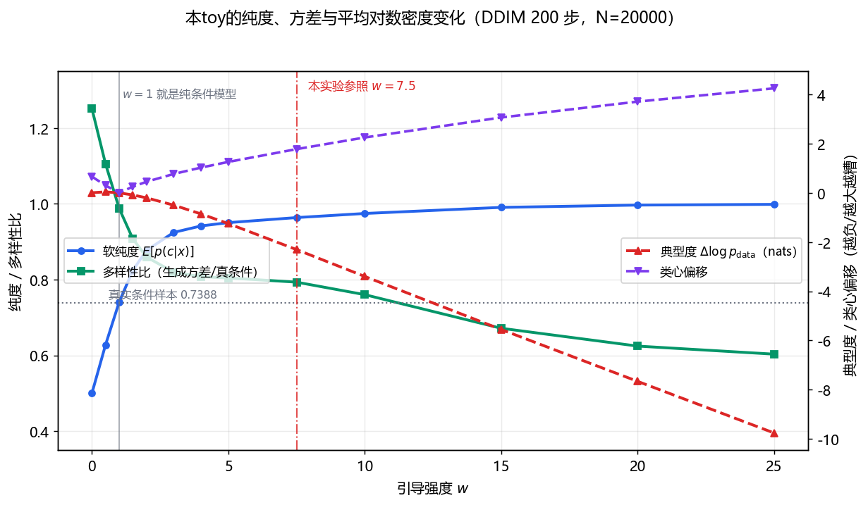
图中比较软纯度、方差比、平均对数密度差和均值偏移。纯度在较小强度处增长较快,其后放缓;其他变化不必线性。$w=7.5$ 是本实验参照点,也是固定Diffusers v0.35.1 StableDiffusionPipeline接口默认值,不能推广至整个SD系列或视频模型。
DDPM 的前向过程写成 $x_t=\sqrt{\bar\alpha_t}x_0+\sqrt{1-\bar\alpha_t}\,\varepsilon$,训练以本次噪声 $\varepsilon$ 作回归目标,平方损失的最优预测是 $E[\varepsilon|x_t,c]$。记
$$e_{\text{c}}=\varepsilon_\theta(x_t,t,c),\qquad e_{\text{un}}=\varepsilon_\theta(x_t,t,\varnothing)$$
其中 $\varnothing$ 是空条件(训练时按一定概率丢弃条件,让同一个权重同时充当两个分支)。CFG 的输出是
$$e_{\text{guided}}=e_{\text{un}}+w\,(e_{\text{c}}-e_{\text{un}})=w\,e_{\text{c}}+(1-w)\,e_{\text{un}}$$
这个改写值得停一下:它是两支预测的仿射组合,系数和为1;在 $w>1$ 时无条件系数为负。$w=1$ 时退化成纯条件分支,$w=0$ 时退化成纯无条件分支,$w>1$ 时无条件分支的系数 $1-w\lt 0$,也就是把「条件相对无条件的优势」往远处推。
常用实现以随机丢弃条件让同一主干学习两支预测;也可分别训练条件与无条件模型。原CFG论文比较过0.1、0.2、0.5的条件丢弃概率,不能当作文生图全系列配置。共享主干通常避免再存一整套网络,空条件embedding是否有额外参数取决于架构;训练仍需分配容量学习空条件任务。原论文写 $(1+w_{\mathrm{paper}})e_{\mathrm{c}}-w_{\mathrm{paper}}e_{\mathrm{un}}$,本文采用Diffusers的 $w=1+w_{\mathrm{paper}}$,引用强度前先统一约定。
先明确精确关系。令 $p_t(x_t|c)$ 为前向加噪后的条件边际,$m_t=E[x_0|x_t,c]$ 为平方损失下最优干净样本预测,$\sigma_t=\sqrt{1-\bar\alpha_t}$。对高斯核求导,再用后验期望提出积分,得到
$$s_t(x_t|c)=\nabla_{x_t}\log p_t(x_t|c)=-\frac{x_t-\sqrt{\bar\alpha_t}m_t}{\sigma_t^2}=-\frac{E[\varepsilon|x_t,c]}{\sigma_t}$$
最优噪声预测器与真实score只差缩放;一般训练网络只有近似关系,向量场也不必恰好是归一化密度的梯度。下面先在精确模型下讨论:
$$\tilde{s}(x_t|c)=\nabla\log p(x_t|\varnothing)+w\big(\nabla\log p(x_t|c)-\nabla\log p(x_t|\varnothing)\big)=(1-w)\nabla\log p(x_t)+w\,\nabla\log p(x_t|c)$$
每个固定噪声时刻定义
$$q_t(z|c)=Z_t^{-1}p_t(z|c)^w p_t(z)^{1-w}$$
$z$ 为该时刻样本,$Z_t$ 为积分归一化常数,不随 $z$ 变化。对真实离散类别,贝叶斯公式给出 $q_t\propto p_t(z)p_t(c|z)^w$;$w\ge0$ 且类别先验非零时,后验有界保证可归一化。任意两个独立模型或负向prompt的密度比需另行检查。其score为
$$\nabla_z\log q_t(z|c)=w\nabla_z\log p_t(z|c)+(1-w)\nabla_z\log p_t(z)$$
两式的梯度相同,但这只是固定时刻的恒等式,不保证所有 $q_t$ 能由同一个 $q_0$ 加噪得到。
关键是时间相容性:「先倾斜再加噪」通常不同于「分别加噪再倾斜」。一个可手算反例是 $p(z|c)=N(0,1)$、$p(z)=N(0,2)$、$w=2$。取 $P(c)=1/2$ 时后验最大为 $\sqrt2/2$,另一类密度取 $2p(z)-p(z|c)$ 非负且积分为1,可构成合法条件/边际对。初始倾斜方差为 $(2-1/2)^{-1}=2/3$;再做 $\bar\alpha_t=1/2$ 的前向加噪,方差为 $5/6$。若先分别加噪,两支方差为1与 $3/2$,再倾斜得到 $(2-2/3)^{-1}=3/4$。两种边际不同,说明score恒等式不能直接推出终点分布;特殊模型可能相等,偏差也未必随强度单调增加。
本toy另从归一化倾斜密度作网格近似采样:$w=7.5$ 时CFG样本与倾斜样本的固定目标交叉熵为3.6926与2.2258 nats,结合均值/方差给出数值反证。交叉熵差不是KL,仍需检查网格与抽样误差,见第08节。
几何上看得更直接:
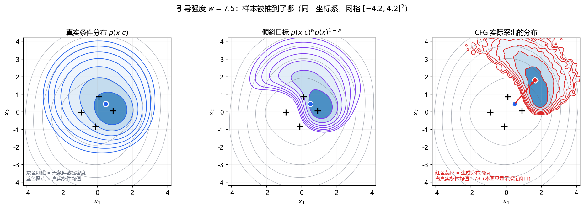
三图为条件密度、归一化倾斜密度和DDIM样本平滑直方图。灰线共用无条件密度标尺,蓝点为真实条件样本均值,右图红点为生成均值,偏移约1.78。窗口仅 $[-4.2,4.2]^2$;直方图丢弃窗外点再在窗口内归一化,不能用颜色比较全部尾部质量,也不能据此量化图像过曝。
设真实的条件/无条件预测为 $e^\star_{\text{c}}$ 与 $e^\star_{\text{un}}$,模型误差为 $\delta_{\text{c}}=e_{\text{c}}-e^\star_{\text{c}}$、$\delta_{\text{un}}=e_{\text{un}}-e^\star_{\text{un}}$。引导后预测相对「同样加权过的真值」$w e^\star_{\text{c}}+(1-w)e^\star_{\text{un}}$ 的误差是
$$\delta_{\text{guided}}=w\,\delta_{\text{c}}+(1-w)\,\delta_{\text{un}}$$
取范数并放缩:
$$\|\delta_{\text{guided}}\|\le w\|\delta_{\text{c}}\|+(w-1)\|\delta_{\text{un}}\|\le(2w-1)\max\big(\|\delta_{\text{c}}\|,\|\delta_{\text{un}}\|\big)$$
这里限定 $w\ge1$,故 $|1-w|=w-1$;一般强度的系数界为 $|w|+|1-w|$。该界比较引导预测相对同样加权真值的误差,不是相对条件预测的误差,也不是端到端分布或画质界。共同误差 $\delta_{\mathrm{c}}=\delta_{\mathrm{un}}$ 会原样保留;相反误差可达到上界;取 $\delta_{\mathrm{un}}=2\delta_{\mathrm{c}}$、$w=2$ 又能完全抵消。实际误差不必随强度单调放大。
外推可能增大预测幅度,但并非必然。中心化逐元素方差满足
$$\operatorname{Var}(e_g)=w^2\operatorname{Var}(e_c)+(1-w)^2\operatorname{Var}(e_u)+2w(1-w)\operatorname{Cov}(e_c,e_u)$$
相关性一个数不足以决定趋势。重建 $\hat x_0=(x_t-\sigma_t e_g)/\sqrt{\bar\alpha_t}$ 还依赖向量方向和噪声档位;标准差大不能直接推出样本远离中心或图像过曝。本文固定探测点上确有幅度增长,作为数值现象报告,Lin等人的图像rescale实验是另一类证据。
核心是「精确去噪器 + DDIM」。高斯混合下 $E[x_0|x_t]$ 有闭式解:分量内部是高斯的,所以
$$E[x_0|x_t,k]=\mu_k+\frac{\bar\alpha_t^{1/2}\,\sigma_k^2}{\bar\alpha_t\sigma_k^2+(1-\bar\alpha_t)}\big(x_t-\bar\alpha_t^{1/2}\mu_k\big)$$
再按分量后验 $r_k=p(k|x_t)$ 加权。代码就是这一行公式:
def x0_hat(X, a_bar, logw):
    s = np.sqrt(a_bar)
    v = a_bar * VAR + (1.0 - a_bar)
    gain = VAR * s / v
    r = posterior(X, a_bar, logw)
    per = MU[None, :, :] + gain[None, :, None] * (X[:, None, :] - s * MU[None, :, :])
    return (r[:, :, None] * per).sum(axis=1)
其中 $k$ 是分量索引,$\mu_k$ 是二维均值,$\sigma_k^2$ 是各向同性方差,$a=\bar\alpha_t$。在分量k内部,高斯条件均值增益是交叉协方差乘观测协方差的逆;各向同性化后其标量系数为
$$g_k=\frac{\sqrt a\sigma_k^2}{a\sigma_k^2+1-a}$$
因此分量后验为
$$r_k=\frac{\pi_k N(x_t;\sqrt a\mu_k,(a\sigma_k^2+1-a)I)}{\sum_j\pi_j N(x_t;\sqrt a\mu_j,(a\sigma_j^2+1-a)I)}$$
再用全期望公式加权。条件分支只把 $\pi_k$ 换成类内归一化先验;这是解析计算,不是训练了一个神经网络。弱分支的各向同性矩匹配应为
$$m=\sum_k\pi_k\mu_k,\qquad v=\frac{1}{d}\sum_k\pi_k\left(d\sigma_k^2+\|\mu_k-m\|^2\right)$$
$d=2$,分量内方差必须先乘维数再平均。条件 $v=0.84$、无条件 $v=1.06625$;它只匹配协方差的迹,不能匹配完整协方差和多模态结构。
这里有个实现上的坑值得单独说:类内重新归一化之后,类外分量的先验变成 0,$\log 0$ 会直接炸。所以所有先验都要先过一遍 safe_log,把非正的权重映到 $-\infty$ 而不是让 numpy 抛 RuntimeWarning。这个坑在写倾斜分布那段还会再咬一次——$\log p_{\text{tilde}}$ 的归一化常数要在网格上做数值积分,网格范围取窄了(比如只取 $\pm3.6$)会把分布的尾巴切掉,归一化常数偏小,后面所有交叉熵都跟着错。本文用的是 $\pm9$ 的 420 点网格。
$\varepsilon$ 预测和 DDIM 的一步:
def eps_hat(X, t, logw):
    a = abar(t)
    return (X - np.sqrt(a) * x0_hat(X, a, logw)) / np.sqrt(1.0 - a)

# DDIM (eta=0) 的一步,含 CFG 与引导区间
e_un = fn(X, t, LOGW_UNCOND)
e_c = fn(X, t, LOGW_COND)
w_eff = w if (lo <= t / T <= hi) else 1.0
e_g = e_un + w_eff * (e_c - e_un)
x0 = (X - np.sqrt(1.0 - a) * e_g) / np.sqrt(a)
X = np.sqrt(a_prev) * x0 + np.sqrt(max(1.0 - a_prev, 0.0)) * e_g
五行里三个细节值得说:
w_eff 那一行的 t / T 是归一化时间索引,区间外直接退回 $w=1$(不是 $w=0$)。这是本教学实现的区间开关;是否跳过参考支另见第06节。e_g 可以写成 w_eff * e_c + (1 - w_eff) * e_un,两者数值等价但后者在 $w$ 很大时更容易看出负系数——建议保留后者以免误读。先验证去噪器本身是对的。做法是数值积分对拍:固定 20 万真实样本,对每个探测点 $x_t$ 按 $q(x_t|x_0)$ 加权求样本平均,跟闭式解比。
[Q1] 精确去噪器 E[x0|xt] 的数值积分对拍
  t     alpha_bar    闭式解 E[x0]        数值积分 E[x0]       最大绝对差
    1  9.999000e-01  [-0.80383,-0.00497]  [-0.80352,-0.00542]   3.00e-02
   50  9.710157e-01  [+0.33377,-0.32706]  [+0.33434,-0.32566]   1.13e-02
  200  6.590385e-01  [-1.63345,-1.01052]  [-1.62640,-1.00988]   1.32e-02
  500  7.858724e-02  [-0.03520,+0.23795]  [-0.03229,+0.24075]   1.03e-02
  900  2.752059e-04  [+0.01798,-0.00712]  [+0.02195,-0.00467]   4.12e-03
 1000  4.035830e-05  [+0.00501,-0.00579]  [+0.00899,-0.00330]   4.03e-03
这些重要性采样结果与闭式解相容,但误差随噪声变化不能证明公式正确:低噪声时权重可能集中到极少数样本。闭式解的依据是上述高斯条件公式;独立对数密度有限差分验证score/MMSE关系,最大绝对差约 $1.17\times10^{-10}$。附录cfg_checks.py也核对矩匹配、倾斜归一化和实际步数。
再验证采样器步数够不够($w=7.5$):
  steps    软纯度    多样性比    典型度      类心偏移
     50     0.9640    0.7490     -2.2718      1.7794
    100     0.9637    0.7782     -2.2930      1.7803
    200     0.9636    0.7933     -2.3042      1.7809
    400     0.9635    0.8006     -2.3101      1.7814
   1000     0.9635    0.8055     -2.3136      1.7815
这些是同一批起点、不同积分网格的敏感性检查;400步现恰好执行400步,原先整除步长会误执行500步。1000步仍不是连续时间真值。后文保留200步口径;不能用单项变化小来声称整个采样器已精确收敛。
参考实现:
StableDiffusionPipeline.__call__以固定Diffusers v0.35.1源码为准,去噪循环里的核心是这几行:
# expand the latents if we are doing classifier free guidance
latent_model_input = torch.cat([latents] * 2) if self.do_classifier_free_guidance else latents
if hasattr(self.scheduler, "scale_model_input"):
    latent_model_input = self.scheduler.scale_model_input(latent_model_input, t)

noise_pred = self.unet(latent_model_input, t, encoder_hidden_states=prompt_embeds,
                       timestep_cond=timestep_cond, cross_attention_kwargs=self.cross_attention_kwargs,
                       added_cond_kwargs=added_cond_kwargs, return_dict=False)[0]

if self.do_classifier_free_guidance:
    noise_pred_uncond, noise_pred_text = noise_pred.chunk(2)
    noise_pred = noise_pred_uncond + self.guidance_scale * (noise_pred_text - noise_pred_uncond)

if self.do_classifier_free_guidance and self.guidance_rescale > 0.0:
    noise_pred = rescale_noise_cfg(noise_pred, noise_pred_text, guidance_rescale=self.guidance_rescale)

latents = self.scheduler.step(noise_pred, t, latents, **extra_step_kwargs, return_dict=False)[0]
和我的最小实现比,有四处差异,每一处都有理由:
第一,合批不等于只启动一个 kernel。 torch.cat 让一次 UNet 调用同时处理两分支,但网络仍包含很多算子、kernel 和临时张量。理论算术量约翻倍;实际延迟与吞吐取决于 batch、显存、并行和硬件,不能直接断言延迟只涨 30%~60% 或吞吐必然减半。
第二,do_classifier_free_guidance 是一个属性而不是参数:
@property
def do_classifier_free_guidance(self):
    return self._guidance_scale > 1 and self.unet.config.time_cond_proj_dim is None
固定实现对 $w\le1$(包括0)都关闭双分支,输出普通条件预测;不能靠把该接口设0复现本文公式的无条件端点。负向embedding也可由调用者预先准备,不能说它在一切情况下从未构造。第二个条件说明带guidance embedding的配置另有路径;LCM、LCM-LoRA和其他少步模型应按实际配置判断。
第三,rescale_noise_cfg 把缩放做成了插值而不是替换:
std_text = noise_pred_text.std(dim=list(range(1, noise_pred_text.ndim)), keepdim=True)
std_cfg = noise_cfg.std(dim=list(range(1, noise_cfg.ndim)), keepdim=True)
noise_pred_rescaled = noise_cfg * (std_text / std_cfg)
noise_cfg = guidance_rescale * noise_pred_rescaled + (1 - guidance_rescale) * noise_cfg
Lin等人原论文3.4节已包含标准差重缩放与 $\phi$ 插值,并报告其配置下 $w=7.5,\phi=0.7$ 效果较好;插值不是Diffusers额外发明的机制。固定SD和SDXL接口的guidance_rescale默认均为0。统计按每样本跨通道/空间维度求,PyTorch std默认作样本方差校正;缩放整个向量,并未先去均值。原函数无分母下界:常量预测可产生0/0或非有限值,移植时须明确跳过/夹紧策略,并记录该策略改变了退化输入定义。
原rescale函数、属性及原 __call__ 中的CFG算术块已在CPU执行,和独立参考误差为 $4.44\times10^{-16}$ 与 $7.11\times10^{-15}$;没有运行完整pipeline或图像checkpoint。
第四,负向prompt走同一个条件通道。 参考支可由空文本换成负向文本,此时它是另一条件预测,不是真正无条件边际的score。组合公式保留,前述贝叶斯后验的密度解释需改写;「不要什么」是操作意图,公式不保证指定语义必被删除。
保留受SD通道尺度启发的简化卷积表来说明固定计算图上batch翻倍。它合并了不同残差块的通道、省略真实上下采样细节,不是实际UNet清单,绝对量不能称为真实模型的MAC下限或参数量。
示意表,64×64潜空间、每元素2字节
单分支:MAC 1.898e11;逐层输入输出字节和0.126 GiB
双分支:MAC 3.796e11;逐层输入输出字节和0.251 GiB
示意卷积权重约517.0 M,权重不因batch翻倍
单层公式为 $\mathrm{MAC}=B H_o W_o C_i C_o k^2$,$H_o,W_o$ 为输出高宽,$C_i,C_o$ 为输入输出通道,$k$ 为方形核边长;一次乘加计一个MAC,按乘法和加法分别计FLOPs时主体约为两倍MAC。逐层字节和不是峰值显存或DRAM流量的上下界:权重共享、串行分支复用、残差暂存、工作区和融合都会影响真实占用。1 GiB为 $2^{30}$ 字节。
修正im2col先把窗口转成 $(B,H,W,C,k_h,k_w)$,再展平每位置的卷积核;直接reshape会混淆空间与核维度。逐索引卷积及PyTorch conv2d均对拍通过。下为本机float32、64×64×320→320、3×3卷积计时,预热一次、5次取最小,包括展平和分配:
batch=1 : 0.1469 s
batch=2 : 0.2883 s
时间比  : 1.9630
串行是两次网络调用,合批是一次batch翻倍的调用;两者均为两个样本级前向当量。50步对应50对100个当量,合批仍是50次UNet调用。CPU/GPU延迟、吞吐和峰值显存须实测,单个卷积时间比不构成完整模型瓶颈证明。
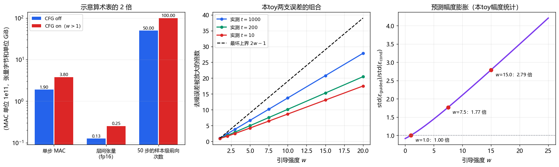
左图倍数只来自示意账本;中图分母为逐点两支误差较大范数的平均,与 $2w-1$ 界一致;右图是在固定探测点上的预测幅度统计。不同图使用各自记录的探测随机流,不应强行对齐最后几位。
探测点固定为「真实数据前向扩散到 $t$」,与 $w$ 无关,这样排除轨迹漂移的干扰:
| $t$ | $w=1$ | $w=2$ | $w=3$ | $w=5$ | $w=7.5$ | $w=15$ |
|---|---|---|---|---|---|---|
| 1000 | 1.000 | 2.411 | 3.824 | 6.651 | 10.186 | 20.791 |
| 700 | 1.000 | 2.403 | 3.808 | 6.620 | 10.136 | 20.685 |
| 400 | 0.986 | 2.198 | 3.429 | 5.899 | 8.991 | 18.271 |
| 200 | 0.952 | 1.915 | 2.925 | 4.974 | 7.551 | 15.302 |
| 50 | 0.896 | 1.666 | 2.518 | 4.276 | 6.502 | 13.217 |
| 10 | 0.890 | 1.639 | 2.473 | 4.198 | 6.384 | 12.983 |
所有列现使用同一分母 $E[\max(\|\delta_c\|,\|\delta_u\|)]$,因此可与对应界1、3、5、9、14、29直接比较。表格只报告此toy探测批结果,不把预测相关系数当作误差相关系数,也不由小t的趋势推导所有模型更易失稳。相反/共同误差与完全抵消反例见第03节和附录。
$t=300$ 处,探测点来自真实条件样本:
| $w$ | 标准差比 |
|---|---|
| 0.0 | 0.9110 |
| 1.0 | 1.0000 |
| 2.0 | 1.1009 |
| 3.0 | 1.2109 |
| 5.0 | 1.4493 |
| 7.5 | 1.7690 |
| 10.0 | 2.1026 |
| 15.0 | 2.7914 |
| 25.0 | 4.2052 |
本探测批的标准差比由0.9110升至4.2052;它是整批二维坐标的统计,不是图像逐样本统计。不能仅凭无条件分支覆盖更多分量就推导其幅度更小,均值、协方差与探测分布共同决定结果。
下面只做二维 toy 的 batch 标准差线性 rescale,在 $w=15$ 下扫系数 $\phi$。真实图像实现按每个样本的 C/H/W 统计;二维向量只有两个坐标,不能把此处整批统计量当成原论文的逐样本实现:
| $\phi$ | 多样性比 | 典型度 | 软纯度 |
|---|---|---|---|
| 0.0 | 0.6716 | −5.5530 | 0.9905 |
| 0.3 | 0.8274 | −6.1435 | 0.9910 |
| 0.5 | 0.9513 | −6.5778 | 0.9913 |
| 0.7 | 1.0944 | −7.0504 | 0.9914 |
| 1.0 | 1.3521 | −7.8447 | 0.9916 |
本toy方差比上升,但平均对数密度差更负;它不能替代真实图像的逐样本rescale实验。若预测乘 $k$,重建改变量为
$$\Delta\hat x_0=(1-k)\frac{\sigma_t}{\sqrt{\bar\alpha_t}}e_g$$
方向由 $e_g$ 决定,取相反预测就得到相反改变量,不能一般说成「把样本往噪声推」。本实验也无像素或感知指标,不能据此声称已修复过曝。
把 $w=7.5$ 只开在归一化噪声档位 $t/T$ 的某个区间内(区间外退回 $w=1$):
| 区间($t/T$) | 软纯度 | 多样性比 | 典型度 | 类心偏移 | 说明 |
|---|---|---|---|---|---|
| $[0.0,1.0]$ | 0.9636 | 0.7933 | −2.3042 | 1.7809 | 全程开 |
| $[0.5,1.0]$ | 0.9126 | 0.9571 | −0.8896 | 0.9365 | 只在高噪声段(链首) |
| $[0.2,0.8]$ | 0.9594 | 0.8167 | −2.0693 | 1.6609 | 只在中段 |
| $[0.0,0.5]$ | 0.9519 | 0.7672 | −1.1345 | 1.2251 | 只在低噪声段(链尾) |
| $[0.0,0.2]$ | 0.9042 | 0.8172 | −0.0831 | 0.4222 | 只在极低噪声段 |
| $[0.0,0.0]$ | 0.7409 | 0.9876 | +0.0030 | 0.0075 | 全程不开($w=1$ 基线) |
再细扫两族区间,用「纯度增益 / 典型度代价」当性价比:
细扫 A:只开链尾(区间 = [0, hi])
  区间        纯度增益    典型度代价    性价比    类心偏移   多样性比
  [0.0,0.1]     +0.0829      0.0099       8.345     0.1649    0.8899
  [0.0,0.2]     +0.1632      0.0861       1.896     0.4222    0.8172
  [0.0,0.3]     +0.1921      0.3080       0.624     0.6888    0.7890
  [0.0,0.4]     +0.2040      0.6816       0.299     0.9630    0.7737
  [0.0,0.5]     +0.2110      1.1375       0.185     1.2251    0.7672
  [0.0,0.8]     +0.2211      2.1335       0.104     1.7045    0.7862
  [0.0,1.0]     +0.2226      2.3072       0.097     1.7809    0.7933

细扫 B:只开链首(区间 = [lo, 1.0])
  区间        纯度增益    典型度代价    性价比    类心偏移   多样性比
  [0.0,1.0]     +0.2226      2.3072       0.097     1.7809    0.7933
  [0.3,1.0]     +0.2154      2.0350       0.106     1.6224    0.8669
  [0.5,1.0]     +0.1716      0.8926       0.192     0.9365    0.9571
  [0.7,1.0]     +0.0674      0.1837       0.367     0.2866    0.9813
  [0.9,1.0]     +0.0101      0.0209       0.481     0.0438    0.9868
本toy只开链尾10%时纯度增益约0.0829、平均对数密度损失约0.0099,比值约8.345。比值带每nat单位,分母近零时敏感;它不是统一质量指标或计算效率。比值最低的点未必被其他点帕累托支配,因为它可能同时取得最高纯度。区间效果不可简单相加,沿途轨迹会改变。
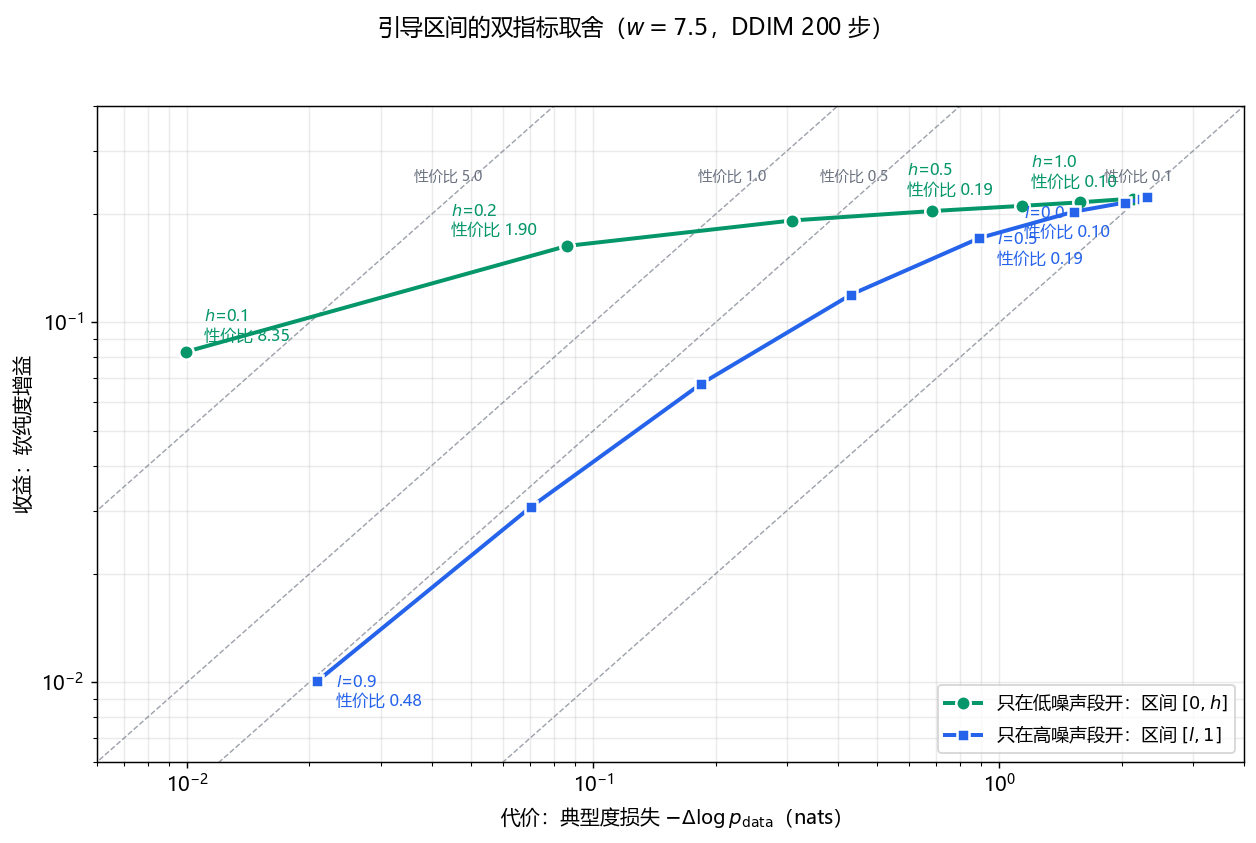
横轴为相对无引导基线的平均对数密度损失,纵轴为软纯度增益,虚线只是固定比值线。两族仅描述本toy的离散候选,不证明完整帕累托前沿。换模型后若增益或代价非正、接近零,双对数图与比值都需调整。
原论文的图像实验发现高噪声引导可能有害、低噪声多余、中段更有用;本toy的指标偏好链尾,不能直接对齐。这里只说明区间值得检验,不能推出所有模型全程引导必非最优。当前教学代码在区间外仍计算两支再设 $w=1$,只改区间并未省算力;生产实现若跳过参考支,$S$步仅 $G$步引导可由 $2S$ 降至 $S+G$ 个当量。$t/T$ 是时间索引比例,不等于标准差或SNR比例,也不是原论文噪声区间的直接坐标。
step_distillation 那篇要展开的内容。这些工作分别处理引导组合、噪声日程与rescale、引导区间、参考模型选择及引导蒸馏,并非所有模型必经的单一替代链。专门训练可减少推理步骤/分支,但会增加训练与适用范围上的约束,不能说所有少步模型都把同一个w作为输入。
误解一:「CFG 就是在采样 $p(x|c)^w p(x)^{1-w}$。」 精确score在固定时刻恒等,最终分布层面不能由此保证。参考统计量是交叉熵 $-E_{X\sim Q}[\log P(X)]$。不同列目标不同,不能横向比较“越小越像”;即使固定 $P$,较低交叉熵也可能来自模式坍缩,需与均值、方差或分布距离联读:
下表 $H_c,H_t,H_u$ 分别为以条件、倾斜和无条件密度作目标的交叉熵,单位nats;后表保留同一批样本的矩统计。
| 强度/来源 | $H_c$ | $H_t$ | $H_u$ |
|---|---|---|---|
| 真实条件 | 2.5757 | — | 2.8562 |
| 1.0/CFG | 2.5670 | 2.5670 | 2.8532 |
| 1.0/倾斜 | 2.5891 | 2.5891 | 2.8706 |
| 3.0/CFG | 2.7405 | 2.4039 | 3.3536 |
| 3.0/倾斜 | 2.4824 | 2.3227 | 3.0070 |
| 7.5/CFG | 4.5048 | 3.6926 | 5.1605 |
| 7.5/倾斜 | 2.6350 | 2.2258 | 3.2287 |
| 15.0/CFG | 7.7257 | 6.1882 | 8.4092 |
| 15.0/倾斜 | 2.9792 | 2.2782 | 3.6030 |
| 强度/来源 | 方差比 | 均值偏移 |
|---|---|---|
| 真实条件 | 1.0000 | 0.0000 |
| 1.0/CFG | 0.9876 | 0.0075 |
| 1.0/倾斜 | 1.0090 | 0.0096 |
| 3.0/CFG | 0.8193 | 0.7721 |
| 3.0/倾斜 | 0.8944 | 0.3546 |
| 7.5/CFG | 0.7933 | 1.7809 |
| 7.5/倾斜 | 0.9077 | 0.6028 |
| 15.0/CFG | 0.6716 | 3.0681 |
| 15.0/倾斜 | 1.0059 | 0.8828 |
$w=1$ 两行有限统计接近,不证明同分布。$w=7.5$ 固定目标交叉熵差约1.47 nats,结合均值偏移1.78对0.60支持本设定中分布不同。log-sum-exp保留归一化偏移;420与840网格的log常数差小于 $1.3\times10^{-14}$,$w=1$ 对数密度恒等误差约 $3.1\times10^{-14}$。这是指定窗口内的数值敏感性检查,不是尾部误差严格界;第03节的解析方差反例不依赖本表抽样。
误解二:「w越大越准。」 必须先定义「准」是条件一致性、覆盖、概率拟合还是观感,不能用一列替代所有目标。
误解三:「没有第二套主干参数,就没有推理成本。」 两支增加样本级当量;示意表MAC由 $1.898\times10^{11}$ 增至 $3.796\times10^{11}$,不等于实际延迟或显存必翻倍。
误解四:「w调小一点就省算力。」 固定双分支配置中由30改成1.01不减少当量;真正关闭参考支或跳过部分步骤才会减少计算,条件计算模型还须检查实际路径。
误解五:「rescale修好了分布,可以无限加w。」 它匹配一种标准差并插值,不保证拟合真实分布;本toy不能替代原论文图像实验。
误解六:「w小于1就是条件采样变弱。」 公式中 $0\lt w\lt 1$ 为预测插值,不是分布混合;固定SD接口对 $w\le1$ 关闭双分支,不能靠把接口设0复现toy的无条件端点。
五个小实验,脚本在附录里,全部只依赖 numpy 与 matplotlib。
实验一:独立验证。 先跑cfg_checks.py,以高斯矩、密度有限差分和逐索引卷积核对公式/代码;再看Q1重要性采样,理解小t权重退化,不把误差趋势当正确性证明。
实验二:扫自己的w。 修改SPECS,保持方差为正并归一化权重,比较同一起点的Q2统计。必要时换seed并增加样本,分别观察条件一致性、方差和密度,不要求新模型复现本文曲线。
实验三:扫引导区间。 记录Q5增益与代价的绝对量,检查近零分母;要量计算收益,须真正跳过区间外参考支并核对调用数,指标比值不能替代吞吐。
实验四:算真实模型。 CONVS只演示固定图随batch的变化。实际UNet账本应由真实模块形状导出,区分权重、同时活跃张量、工作区与硬件计时;修改示意表几行不保证得到模型下限。
实验五:构造反例。 cfg_checks.py检查先倾斜/先加噪的5/6与3/4方差、误差保持/达到界/抵消,以及rescale改变量方向可相反。先核对边界,再在真实模型评估画质。
读这篇之前建议先看:
读完之后:
回到知识树:本文是「生成范式」方向的一级节点,往上接 DDPM,往下接少步蒸馏。
09 节用到的脚本全文如下(cfg_checks.py、cfg_gmm.py、cfg_lab.py、make_figures.py)。复制到本地存成同名文件,按各脚本开头的依赖说明准备环境后即可运行。
"""Independent CFG algebra, moment, convolution and numerical-boundary checks (NumPy only)."""
import json
from pathlib import Path
import numpy as np
import cfg_gmm as G
import cfg_lab as L


def validate():
    rng = np.random.default_rng(20261020)
    moment_errors = []
    for logw in [G.LOGW_COND, G.LOGW_UNCOND]:
        w = np.exp(logw); w /= w.sum()
        mean = w @ G.MU
        cov = sum(w[k]*(G.VAR[k]*np.eye(G.DIM)+np.outer(G.MU[k]-mean,G.MU[k]-mean)) for k in range(G.K))
        m,v = G.single_gauss(logw)
        moment_errors += [float(np.max(np.abs(m-mean))),float(abs(v-np.trace(cov)/G.DIM))]
    # Direct index convolution checks avoid reproducing im2col's axis order.
    x = rng.normal(size=(2,2,4,5)); w = rng.normal(size=(3,2,3,3))
    padded = np.pad(x,((0,0),(0,0),(1,1),(1,1)))
    expected = np.zeros((2,3,4,5))
    for n in range(2):
        for co in range(3):
            for h in range(4):
                for j in range(5):
                    expected[n,co,h,j] = np.sum(padded[n,:,h:h+3,j:j+3]*w[co])
    conv_error = float(np.max(np.abs(L.conv3x3(x,w)-expected)))
    # Finite-difference log-mixture gradients independently verify MMSE-score identity.
    X = rng.normal(size=(30,2)); score_errors=[]
    for t in [1,200,900]:
        a = G.abar(t); h = 1e-5
        for logw in [G.LOGW_COND,G.LOGW_UNCOND]:
            def lp(q):return G.logsumexp_rows(G.logpdf_comps(q,a)+logw[None,:])
            grad = np.column_stack([(lp(X+h*np.eye(2)[i])-lp(X-h*np.eye(2)[i]))/(2*h) for i in range(2)])
            pred = -G.eps_hat(X,t,logw)/np.sqrt(1-a)
            score_errors.append(float(np.max(np.abs(pred-grad))))
    # p_u=N(0,2), p_c=N(0,1) can be genuine marginals: prior p(c)=1/2 bounds p(c|x)<=sqrt(2)/2.
    # w=2 gives tilted variance 2/3 at t=0; alpha_bar=1/2 yields 5/6 after forward noise,
    # whereas tilting the separately noised branches gives 3/4.
    tilted0 = 1/(2/1-1/2); forward = 0.5*tilted0+0.5
    tilted_t = 1/(2/(0.5*1+0.5)-1/(0.5*2+0.5))
    # Error cancellation and tightness do not require Monte Carlo or trained models.
    dc,du = np.array([1.,-2.]), np.array([-1.,2.])
    tight_error = abs(np.linalg.norm(3*dc-2*du)-5*np.linalg.norm(dc))
    cancel = 2*np.array([1.,0.])-np.array([2.,0.])
    # Rescaling epsilon by k changes x0 by +(1-k)*sqrt((1-a)/a)*epsilon, whose direction is not fixed.
    a,k = 0.5,0.5
    delta = [float((1-k)*np.sqrt((1-a)/a)*eps) for eps in [-2.,2.]]
    grid = {}
    for wval in [1.,7.5,15.]:
        values=[]
        for n in [420,840]:
            G.logp_tilt_norm(np.zeros((1,2)),wval,n=n)
            values.append(G._TILT_CACHE[(wval,-9.,9.,n)])
        grid[str(wval)] = dict(logZ=values,absolute_difference=abs(values[0]-values[1]))
    identity = float(np.max(np.abs(G.logp_tilt_norm(X,1.)-G.logp_cond(X))))
    counts={str(s):len(G.ddim_timesteps(s)) for s in [1,50,200,400,1000]}
    assert max(moment_errors)<1e-12 and conv_error<1e-12 and max(score_errors)<1e-7
    assert abs(forward-5/6)<1e-12 and abs(tilted_t-3/4)<1e-12 and tight_error<1e-12
    assert np.linalg.norm(cancel)==0 and identity<1e-10
    assert all(int(k)==v for k,v in counts.items())
    result=dict(passed=True,moment_max_error=max(moment_errors),conditional_isotropic_variance=G.single_gauss(G.LOGW_COND)[1],
                unconditional_isotropic_variance=G.single_gauss(G.LOGW_UNCOND)[1],convolution_max_error=conv_error,
                score_finite_difference_max_error=max(score_errors),time_compatibility_counterexample=dict(initial_tilt_variance=tilted0,forward_tilt_variance=forward,tilt_noised_variance=tilted_t),
                error_bound_tightness_error=tight_error,error_cancellation_norm=float(np.linalg.norm(cancel)),rescale_x0_delta_opposite_signs=delta,
                tilt_grid_convergence=grid,w1_normalization_error=identity,timestep_counts=counts,errors=[],warnings=[])
    return result

if __name__ == '__main__':
    result=validate()
    Path(__file__).with_name('validation_results.json').write_text(json.dumps(result,ensure_ascii=False,indent=2),encoding='utf-8')
print(json.dumps(result,ensure_ascii=False,indent=2))# -*- coding: utf-8 -*-
"""cfg_gmm.py —— 在一个「去噪器可解析求解」的高斯混合模型上把 CFG 做实。
为什么非要用 GMM:
CFG 需要一支条件去噪器和一支无条件去噪器。用真网络的话两支都有训练误差,
观察到的形变会混入模型误差。而 GMM 的 MMSE 去噪器
E[x0|xt] 有闭式解,两支都是**精确**的,但采样仍有有限步、起点和有限样本误差。
另外 p_t(x_t|c) 也有解析式,可以直接验证「CFG 是不是在从倾斜分布
p(x|c)^w p(x)^{1-w} 里采样」这个命题。
本脚本回答六个问题(全部是实跑数字,不是推测):
Q1 精确去噪器对不对?(数值积分对拍)
Q2 w 扫描:条件纯度 / 多样性 / 典型度 怎么变?
Q3 CFG 采出来的分布,是不是那个倾斜分布?
Q4 w 把去噪器的**误差**放大了多少倍?(最坏上界 2w-1)
Q5 只在某个噪声区间开引导,比全程开好吗?
Q6 引导后的预测幅度膨胀多少?rescale 能不能压回去?
运行: /usr/local/bin/python3 cfg_gmm.py
依赖: numpy(无 torch,全部闭式解 + 向量化)
"""
import numpy as np
# ═════════════════════════════ 1. 数据:两组、四个高斯分量 ═════════════════════════════
# (均值, 各向同性方差, 无条件权重, 类别标签)
# 设计意图:两类故意重叠(类心相距约 1.3,分量标准差 0.6~1.0),
# 这样 w=1 时条件采样仍会「漏」到对面,给 CFG 留出可观测的改善空间。
# 两类各有一个「紧」分量和一个「松」分量 —— 方差不齐是后面「模式漂进尾巴」的关键。
SPECS = [
((-0.90, -0.05), 0.36, 0.25, 0),
((-0.10, -0.85), 1.00, 0.25, 0),
((0.90, 0.05), 0.36, 0.25, 1),
((0.10, 0.85), 1.00, 0.25, 1),
]
MU = np.array([s[0] for s in SPECS], dtype=float) # [K, 2]
VAR = np.array([s[1] for s in SPECS], dtype=float) # [K]
PI = np.array([s[2] for s in SPECS], dtype=float) # [K]
CLS = np.array([s[3] for s in SPECS], dtype=int) # [K]
K = len(SPECS)
DIM = 2
TARGET_CLS = 1 # 本文统一用「条件 = 类别 1」做演示
# ── 调度:DDPM 线性 beta,T=1000(与 ddpm 那篇同一套口径)──
T = 1000
BETAS = np.linspace(1e-4, 0.02, T)
ALPHAS = 1.0 - BETAS
ABAR = np.cumprod(ALPHAS) # alpha_bar,下标 0 对应 t=1
def abar(t):
"""alpha_bar_t,t 从 1 开始(与论文记号一致)。"""
return ABAR[t - 1]
def safe_log(w):
"""对数,0 分量记为 -inf 而不报警告。"""
w = np.asarray(w, dtype=float)
out = np.full_like(w, -np.inf)
m = w > 0
out[m] = np.log(w[m])
return out
# ═════════════════════════════ 2. 精确去噪器 ═════════════════════════════
def logpdf_comps(X, a_bar):
"""每个分量对 x_t 的对数密度:x_t|k ~ N(sqrt(a) mu_k, a var_k + (1-a))。"""
s = np.sqrt(a_bar)
m = s * MU # [K, 2]
v = a_bar * VAR + (1.0 - a_bar) # [K]
d2 = ((X[:, None, :] - m[None, :, :]) ** 2).sum(-1) # [N, K]
return -0.5 * (d2 / v[None, :] + DIM * np.log(2 * np.pi * v)[None, :])
def posterior(X, a_bar, logw):
"""分量后验权重 r_k = p(k | x_t)。logw 是分量的对数先验。"""
lp = logpdf_comps(X, a_bar) + logw[None, :]
lp -= lp.max(axis=1, keepdims=True)
r = np.exp(lp)
return r / r.sum(axis=1, keepdims=True)
def x0_hat(X, a_bar, logw):
"""MMSE 估计 E[x0 | x_t](精确闭式解)。
分量内部是高斯的,所以 E[x0|x_t,k] 有闭式解:
mu_k + S_k sqrt(a) (a S_k + (1-a) I)^{-1} (x_t - sqrt(a) mu_k)
再按后验权重 r_k 加权。S_k = var_k * I,所以增益是个标量。
"""
s = np.sqrt(a_bar)
v = a_bar * VAR + (1.0 - a_bar)
gain = VAR * s / v # [K]
r = posterior(X, a_bar, logw) # [N, K]
per = MU[None, :, :] + gain[None, :, None] * (X[:, None, :] - s * MU[None, :, :])
return (r[:, :, None] * per).sum(axis=1) # [N, 2]
def eps_hat(X, t, logw):
"""epsilon 预测:eps = (x_t - sqrt(a) x0_hat) / sqrt(1-a)。"""
a = abar(t)
return (X - np.sqrt(a) * x0_hat(X, a, logw)) / np.sqrt(1.0 - a)
def cond_logw(cls):
"""条件分支的分量对数先验:只保留该类内部分量,类内权重重新归一化。"""
w = np.where(CLS == cls, PI, 0.0)
w = w / w.sum()
return safe_log(w)
LOGW_UNCOND = safe_log(PI) # 无条件:全混合
LOGW_COND = cond_logw(TARGET_CLS) # 条件:类别 TARGET_CLS
# ── 弱去噪器:把整簇拟合成「一个高斯」之后的线性维纳滤波 ──
# 给 Q4 用的「不完美模型」:它是该高斯下的最优线性去噪器,但真实数据是混合体,
# 所以误差非零、且随 t 变化 —— 正好用来看 w 的放大倍数。
def single_gauss(logw):
"""按分量权重算出混合体的均值与平均方差。"""
w = np.exp(logw)
w = w / w.sum()
mu = (w[:, None] * MU).sum(0)
var = (w * (DIM * VAR + (MU ** 2).sum(1))).sum() - (mu ** 2).sum()
return mu, var / DIM
def weak_eps_hat(X, t, logw):
"""单高斯近似的线性去噪器(有误差)。"""
a = abar(t)
mu, var = single_gauss(logw)
s = np.sqrt(a)
v = a * var + (1.0 - a)
gain = var * s / v
x0 = mu[None, :] + gain * (X - s * mu[None, :])
return (X - s * x0) / np.sqrt(1.0 - a)
# ═════════════════════════════ 3. 采样器(DDIM, eta=0) ═════════════════════════════
def ddim_timesteps(steps):
"""均匀步长的 DDIM 时间步序列,从 T 递减;末次直接到干净端,调用数恰为 steps。"""
if not isinstance(steps, int) or not 1 <= steps <= T:
raise ValueError("steps must be an integer in [1,T]")
if T % steps == 0:
return list(range(T, 0, -(T // steps)))
return np.linspace(T, 1, steps).round().astype(int).tolist()
def ddim_sample(x_T, steps=200, w=1.0, interval=(0.0, 1.0),
weak=False, rescale=0.0):
"""确定性 DDIM 采样(eta=0),带 CFG。
x_T : [N, 2] 纯噪声起点
w : 引导强度(w=1 即纯条件,w=0 即纯无条件)
interval : 引导生效的 t/T 区间 (lo, hi)。区间外退化为 w=1。
weak : True 则用单高斯弱去噪器(Q4/Q6 用)
rescale : 二维玩具的 batch 标准差线性 rescale 系数 phi;不等于图像逐样本 rescale
"""
fn = weak_eps_hat if weak else eps_hat
ts = ddim_timesteps(steps)
X = x_T.copy()
lo, hi = interval
for i, t in enumerate(ts):
a = abar(t)
a_prev = abar(ts[i + 1]) if i + 1 < len(ts) else 1.0
e_un = fn(X, t, LOGW_UNCOND)
e_c = fn(X, t, LOGW_COND)
frac = t / T
w_eff = w if (lo <= frac <= hi) else 1.0
e_g = e_un + w_eff * (e_c - e_un) # = w_eff*e_c + (1-w_eff)*e_un
if rescale > 0.0:
# 二维 toy 用整批统计量;图像实现应按样本跨 C/H/W 统计。
# 沿用线性插值,而不是把标准差比取 phi 次幂。
s_g, s_c = e_g.std(), e_c.std()
if s_g > 1e-12:
e_g = (1.0 - rescale) * e_g + rescale * e_g * (s_c / s_g)
x0 = (X - np.sqrt(1.0 - a) * e_g) / np.sqrt(a)
X = np.sqrt(a_prev) * x0 + np.sqrt(max(1.0 - a_prev, 0.0)) * e_g
return X
# ═════════════════════════════ 4. 度量 ═════════════════════════════
def logsumexp_rows(lp):
m = lp.max(axis=1, keepdims=True)
return m[:, 0] + np.log(np.exp(lp - m).sum(axis=1))
def logp_data(X):
"""真实数据分布(无条件 GMM)的对数密度。"""
return logsumexp_rows(logpdf_comps(X, 1.0) + safe_log(PI)[None, :])
def logp_cond(X):
"""真实条件分布 p(x|c=TARGET_CLS) 的对数密度。"""
return logsumexp_rows(logpdf_comps(X, 1.0) + LOGW_COND[None, :])
def class_posterior(X):
"""p(类别=TARGET_CLS | x) —— 用真实 GMM 算,作为「软纯度」。"""
lp = logpdf_comps(X, 1.0) + safe_log(PI)[None, :]
m = lp.max(axis=1, keepdims=True)
r = np.exp(lp - m)
r /= r.sum(axis=1, keepdims=True)
return (r * (CLS[None, :] == TARGET_CLS)).sum(axis=1)
def spread(X):
"""分布的「宽度」:每维方差的平均。"""
return float(np.mean(X.var(axis=0)))
def summarize(X, Xref, tag=""):
"""一组样本的核心指标。Xref 是真实条件分布 p(x|c) 的样本,作为基准。"""
d2 = ((X[:, None, :] - MU[None, :, :]) ** 2).sum(-1) / VAR[None, :]
return dict(
tag=tag,
purity=float(class_posterior(X).mean()),
hard=float((CLS[np.argmin(d2, axis=1)] == TARGET_CLS).mean()),
div=float(spread(X) / spread(Xref)),
typicality=float(logp_data(X).mean() - logp_data(Xref).mean()),
bias=float(np.linalg.norm(X.mean(0) - Xref.mean(0))),
)
def sample_data(rng, n, cls=None):
"""从真实 GMM 采 n 个样本;cls 非空则只采该类的样本。"""
w = PI.copy()
if cls is not None:
w = np.where(CLS == cls, PI, 0.0)
w = w / w.sum()
k = rng.choice(K, size=n, p=w)
return MU[k] + np.sqrt(VAR[k])[:, None] * rng.standard_normal((n, DIM))
# ═══════════════════════ 5. 倾斜分布 p(x|c)^w p(x)^{1-w} ═══════════════════════
def tilted_logpdf(X, w):
"""未归一化的倾斜对数密度:w*log p(x|c) + (1-w)*log p(x)。"""
return w * logp_cond(X) + (1.0 - w) * logp_data(X)
def _tilt_grid(w, lo=-9.0, hi=9.0, n=420):
"""在方格上算归一化后的倾斜密度,返回 (xs, P[ny, nx]),P 求和为 1。"""
xs = np.linspace(lo, hi, n)
GX, GY = np.meshgrid(xs, xs)
P = np.column_stack([GX.ravel(), GY.ravel()])
lp = tilted_logpdf(P, w)
lp -= lp.max()
d = np.exp(lp).reshape(n, n)
return xs, d / d.sum()
_TILT_CACHE = {}
def logp_tilt_norm(X, w, lo=-9.0, hi=9.0, n=420):
"""归一化后的 log p_tilde(x)(归一化常数由方格数值积分得到)。"""
key = (float(w), float(lo), float(hi), int(n))
if key not in _TILT_CACHE:
xs = np.linspace(lo, hi, n)
GX, GY = np.meshgrid(xs, xs)
lp = tilted_logpdf(np.column_stack([GX.ravel(), GY.ravel()]), w)
offset = lp.max()
d = np.exp(lp - offset).reshape(n, n)
Z = d.sum() * (xs[1] - xs[0]) ** 2
_TILT_CACHE[key] = offset + np.log(Z)
return tilted_logpdf(X, w) - _TILT_CACHE[key]
def sample_tilted(rng, w, n):
"""从倾斜分布 p(x|c)^w p(x)^{1-w} 采样(方格离散近似 + 格内抖动)。"""
xs, d = _tilt_grid(w)
flat = d.ravel()
idx = rng.choice(len(flat), size=n, p=flat / flat.sum())
iy, ix = np.unravel_index(idx, d.shape)
step = xs[1] - xs[0]
return np.column_stack([xs[ix] + (rng.random(n) - 0.5) * step,
xs[iy] + (rng.random(n) - 0.5) * step])
# ═════════════════════════════ 6. 主流程 ═════════════════════════════
def base_rng():
"""主实验与画图共用的随机流起点。
两边必须 draw 相同次数、相同顺序,否则图上的数字和正文表格会对不上。
"""
rng = np.random.default_rng(20260928)
Xref = sample_data(rng, 40000, cls=TARGET_CLS)
return rng, Xref
def main():
rng, Xref = base_rng()
q0_rows = {}; q1_rows = []; weak_rows = {}; rescale_rows = {}
N = 20000
STEPS = 200
print("=" * 78)
print("CFG 实跑账本 —— 数据:2D 高斯混合,4 分量 / 2 类,条件 = 类别 %d" % TARGET_CLS)
print("=" * 78)
# ── Q1:精确去噪器对拍(数值积分) ──
print("\n[Q1] 精确去噪器 E[x0|xt] 的数值积分对拍")
print(" 做法:固定 20 万真实样本,对每个探测点 xt 按 q(xt|x0) 加权求样本平均。")
print(" t alpha_bar 闭式解 E[x0] 数值积分 E[x0] 最大绝对差")
mc_rng = np.random.default_rng(7)
X0 = sample_data(mc_rng, 200000)
for t in (1, 50, 200, 500, 900, 1000):
a = abar(t)
Xt = np.sqrt(a) * X0 + np.sqrt(1 - a) * mc_rng.standard_normal(X0.shape)
idx = mc_rng.integers(0, len(X0), size=60)
xt_probe = Xt[idx]
mc = np.empty_like(xt_probe)
s = np.sqrt(a)
for j, xp in enumerate(xt_probe): # 逐点算,避免大临时矩阵
# 权重就是 q(xt|x0) ∝ exp(-||xt - sqrt(a) x0||^2 / (2(1-a)))
d2 = ((xp[None, :] - s * X0) ** 2).sum(-1)
ww = np.exp(-0.5 * (d2 - d2.min()) / (1 - a)) # 减最小值防下溢
ww /= ww.sum()
mc[j] = (X0 * ww[:, None]).sum(0)
q1_rows.append(dict(t=t, min_ess=float(1.0/(ww@ww))))
cf = x0_hat(xt_probe, a, LOGW_UNCOND) # 探测数据来自全混合,故用无条件先验
print(" %4d %.6e [%+.5f,%+.5f] [%+.5f,%+.5f] %.2e"
% (t, a, cf[0, 0], cf[0, 1], mc[0, 0], mc[0, 1],
np.abs(mc - cf).max()))
print(" → MC差异不能独立证明闭式解正确;小t的重要性权重会退化。独立验证见cfg_checks.py。")
# 基准
print("\n基准:真实条件分布 p(x|c=%d)" % TARGET_CLS)
print(" 每维方差 %.4f | 均值 [%+.4f,%+.4f] | 平均 log p_data %.4f | 软纯度 %.4f"
% (spread(Xref), Xref.mean(0)[0], Xref.mean(0)[1],
logp_data(Xref).mean(), class_posterior(Xref).mean()))
x_T0 = rng.standard_normal((N, DIM))
# ── 步长收敛检查 ──
print("\n[Q0] DDIM 步数收敛检查(w=7.5,看 200 步够不够;1000 步 = 全量 T)")
print(" steps 软纯度 多样性比 典型度 类心偏移")
for st in (50, 100, 200, 400, 1000):
X = ddim_sample(x_T0, steps=st, w=7.5)
m = summarize(X, Xref)
q0_rows[st] = dict(actual_steps=len(ddim_timesteps(st)), **m)
print(" %4d %.4f %.4f %+.4f %.4f"
% (st, m["purity"], m["div"], m["typicality"], m["bias"]))
# ── Q2:w 扫描 ──
print("\n[Q2] 引导强度 w 扫描(精确去噪器,DDIM %d 步,N=%d)" % (STEPS, N))
print(" w 软纯度 硬纯度 多样性比 典型度(nats) 类心偏移")
r0 = summarize(Xref, Xref, tag="真实条件")
print(" 真实条件样本(参照) %.4f %.4f %.4f %+.4f %.4f"
% (r0["purity"], r0["hard"], r0["div"], r0["typicality"], r0["bias"]))
sweep = {}
for w in (0.0, 1.0, 2.0, 3.0, 5.0, 7.5, 10.0, 15.0, 25.0):
X = ddim_sample(x_T0, steps=STEPS, w=w)
m = summarize(X, Xref)
sweep[w] = m
print(" %5.1f %.4f %.4f %.4f %+.4f %.4f"
% (w, m["purity"], m["hard"], m["div"], m["typicality"], m["bias"]))
print(" 软纯度 = E[p(c|x)](真实后验);硬纯度 = 马氏最近分量属于目标类的比例;")
print(" 多样性比 = 生成样本每维方差 / 真实条件方差;")
print(" 典型度 = 生成样本与真实样本的平均 log p_data 之差(负 = 平均落在较低密度区,不代表支撑之外)。")
# ── Q3:CFG 采的是不是倾斜分布 ──
print("\n[Q3] CFG 采出的分布 vs 倾斜目标 p(x|c)^w p(x)^{1-w}")
print(" 统计量:固定目标的交叉熵差可否定同分布;更小不保证更像目标")
print(" w 样本来源 -E[log p(x|c)] -E[log p_tilde] -E[log p(x)] 方差比 类心偏移")
tilt_rows = {}
# 参照行:真实条件分布自己的交叉熵(作为「完美拟合」的刻度)
print(" ---- 真实条件样本 %10.4f %10s %10.4f %6.4f %6.4f"
% (-float(logp_cond(Xref).mean()), "(w=1 时同)",
-float(logp_data(Xref).mean()),
spread(Xref) / spread(Xref),
float(np.linalg.norm(Xref.mean(0) - Xref.mean(0)))))
for w in (1.0, 3.0, 7.5, 15.0):
Xg = ddim_sample(x_T0, steps=STEPS, w=w)
Xt = sample_tilted(rng, w, 20000)
for name, X in (("CFG 生成", Xg), ("倾斜目标", Xt)):
row = dict(
ce_cond=-float(logp_cond(X).mean()),
ce_tilt=-float(logp_tilt_norm(X, w).mean()),
ce_data=-float(logp_data(X).mean()),
div=float(spread(X) / spread(Xref)),
bias=float(np.linalg.norm(X.mean(0) - Xref.mean(0))),
)
tilt_rows[(w, name)] = row
print(" %4.1f %-11s %10.4f %10.4f %10.4f %6.4f %6.4f"
% (w, name, row["ce_cond"], row["ce_tilt"], row["ce_data"],
row["div"], row["bias"]))
print(" ↑ 结合均值和方差判断;仅交叉熵接近不能证明同分布")
# ── Q4:误差放大(固定探测分布) ──
print("\n[Q4] 弱去噪器(单高斯近似)下,w 把误差放大了多少倍")
print(" 探测点固定为「真实数据前向扩散到 t」,与 w 无关,排除轨迹漂移的干扰。")
ws4 = (1.0, 2.0, 3.0, 5.0, 7.5, 15.0)
print(" t " + " ".join("w=%-4g" % w for w in ws4)
+ " 最坏上界 2w-1(同序)")
probe = sample_data(rng, 20000)
amp_by_t = {}
for t in (1000, 700, 400, 200, 50, 10):
a = abar(t)
Xt = np.sqrt(a) * probe + np.sqrt(1 - a) * rng.standard_normal(probe.shape)
ec = weak_eps_hat(Xt, t, LOGW_COND) - eps_hat(Xt, t, LOGW_COND)
eu = weak_eps_hat(Xt, t, LOGW_UNCOND) - eps_hat(Xt, t, LOGW_UNCOND)
base = np.maximum(np.linalg.norm(ec, axis=1), np.linalg.norm(eu, axis=1)).mean()
row = []
for w in ws4:
amp = np.linalg.norm(w * ec + (1.0 - w) * eu, axis=1).mean()
row.append(amp / max(base, 1e-12))
amp_by_t[t] = row
print(" %4d " % t + " ".join("%6.3f" % v for v in row)
+ " " + " ".join("%.0f" % (2 * w - 1) for w in ws4))
print(" → 分母为逐点两支较大误差范数的平均,与2w-1界一致;相关误差可放大也可抵消。")
print("\n 各向同性矩匹配弱去噪器下端到端效果(仅本toy):")
print(" w 生成方差/真条件 软纯度")
for w in ws4:
X = ddim_sample(x_T0, steps=STEPS, w=w, weak=True)
m = summarize(X, Xref)
weak_rows[w] = m
print(" %5.1f %.4f %.4f" % (w, m["div"], m["purity"]))
# ── Q5:引导区间 ──
print("\n[Q5] 只在某个噪声区间开引导(w=7.5,精确去噪器,DDIM %d 步)" % STEPS)
print(" 区间(t/T) 软纯度 多样性比 典型度 类心偏移 说明")
intervals = [
((0.0, 1.0), "全程开"),
((0.5, 1.0), "只在高噪声段(链的前半)"),
((0.2, 0.8), "只在中段"),
((0.0, 0.5), "只在低噪声段(链的后半)"),
((0.0, 0.2), "只在极低噪声段"),
((0.0, 0.0), "全程不开(w=1 基线)"),
]
interval_rows = {}
base = None
for (lo, hi), name in intervals:
if (lo, hi) == (0.0, 0.0):
X = ddim_sample(x_T0, steps=STEPS, w=1.0)
else:
X = ddim_sample(x_T0, steps=STEPS, w=7.5, interval=(lo, hi))
m = summarize(X, Xref)
interval_rows[(lo, hi)] = dict(name=name, **m)
if (lo, hi) == (0.0, 0.0):
base = m
print(" [%.1f,%.1f] %.4f %.4f %+.4f %.4f %s"
% (lo, hi, m["purity"], m["div"], m["typicality"], m["bias"], name))
# 细扫:把「区间末端从哪切」和「区间起点从哪切」分别扫一遍,看帕累托前沿
print("\n 细扫 A:只看链的后半段(区间 = [0, hi]),hi 从 0.1 扫到 1.0")
print(" 区间 纯度增益 典型度代价 性价比 类心偏移 多样性比")
fine_a = {}
for hi in (0.1, 0.2, 0.3, 0.4, 0.5, 0.6, 0.8, 1.0):
X = ddim_sample(x_T0, steps=STEPS, w=7.5, interval=(0.0, hi))
m = summarize(X, Xref)
g = m["purity"] - base["purity"]
c = -(m["typicality"] - base["typicality"])
fine_a[hi] = dict(gain=g, cost=c, ratio=g / c, **m)
print(" [0.0,%.1f] %+.4f %.4f %6.3f %.4f %.4f"
% (hi, g, c, g / c, m["bias"], m["div"]))
print("\n 细扫 B:只看链的前半段(区间 = [lo, 1.0]),lo 从 0.0 扫到 0.9")
print(" 区间 纯度增益 典型度代价 性价比 类心偏移 多样性比")
fine_b = {}
for lo in (0.0, 0.1, 0.2, 0.3, 0.4, 0.5, 0.6, 0.7, 0.8, 0.9):
X = ddim_sample(x_T0, steps=STEPS, w=7.5, interval=(lo, 1.0))
m = summarize(X, Xref)
g = m["purity"] - base["purity"]
c = -(m["typicality"] - base["typicality"])
fine_b[lo] = dict(gain=g, cost=c, ratio=g / c, **m)
print(" [%.1f,1.0] %+.4f %.4f %6.3f %.4f %.4f"
% (lo, g, c, g / c, m["bias"], m["div"]))
# ── Q6:幅度膨胀 + rescale ──
print("\n[Q6] 引导后预测的幅度膨胀(t=300,探测点来自真实条件样本)")
Xp_base = sample_data(rng, 8000, cls=TARGET_CLS)
a300 = abar(300)
Xp = np.sqrt(a300) * Xp_base + np.sqrt(1 - a300) * rng.standard_normal(Xp_base.shape)
e_c = eps_hat(Xp, 300, LOGW_COND)
e_u = eps_hat(Xp, 300, LOGW_UNCOND)
rho = float(np.corrcoef(e_c.ravel(), e_u.ravel())[0, 1])
print(" 两分支预测的相关系数 rho = %.4f(不等于误差相关性或幅度单调性证明)" % rho)
print(" w std(eps_guided)/std(eps_cond)")
infl = {}
for w in (0.0, 1.0, 2.0, 3.0, 5.0, 7.5, 10.0, 15.0, 25.0):
e_g = e_u + w * (e_c - e_u)
infl[w] = float(e_g.std() / e_c.std())
print(" %5.1f %.4f" % (w, infl[w]))
print("\n guidance rescale 的效果(w=15):")
print(" phi 多样性比 典型度 软纯度")
for phi in (0.0, 0.3, 0.5, 0.7, 1.0):
X = ddim_sample(x_T0, steps=STEPS, w=15.0, rescale=phi)
m = summarize(X, Xref)
rescale_rows[phi] = m
print(" %.1f %.4f %+.4f %.4f"
% (phi, m["div"], m["typicality"], m["purity"]))
print(" → 本设定(精确去噪器 + DDIM eta=0)下 rescale 把多样性拉回来了,")
print(" 但典型度更差:它缩放的是 eps 的幅度,而 x0 是 eps 的仿射函数,")
print(" x0的改变量依赖eps向量方向,不可一般解释为往噪声推。")
print("\n" + "=" * 78)
import json
from pathlib import Path
result = dict(seed=20260928, N=N, steps=STEPS, q0=q0_rows, q1_last_probe_ess=q1_rows,
sweep=sweep, weak=weak_rows, error_amplification=amp_by_t,
tilt={str(k):v for k,v in tilt_rows.items()}, intervals={str(k):v for k,v in interval_rows.items()},
fine_a=fine_a, fine_b=fine_b, inflation=infl, rescale=rescale_rows, rho=rho,
reference=summarize(Xref,Xref))
Path(__file__).with_name("experiment_results.json").write_text(json.dumps(result,ensure_ascii=False,indent=2),encoding="utf-8")
print("全部数字由本脚本实跑产生,结构化结果 experiment_results.json。")
print("=" * 78)
if __name__ == "__main__":
main()# -*- coding: utf-8 -*-
"""cfg_lab.py —— CFG 的代价账本:算术量、逐层输入输出字节和、实测耗时。
这一篇的立论是「CFG 让每步算两遍,是推理成本里最容易被忽视的 2×」。
这句话里「2×」是**在固定示意账本口径下精确**的(batch 维翻倍、权重不变),
但读者真正想知道的是:这个 2× 在真机上兑现成多少墙钟时间。
本脚本做三件事:
L1 按 stable-diffusion-v1-5 的 UNet 配置手算一份示意卷积表的算术与张量字节和(fp16),
给出「单步张量字节和」和「单步 MAC」这两个绝对量级。
L2 用 numpy 真跑一个 64x64x320 的 3x3 卷积,实测 batch=1 与 batch=2 的时间比。
(CPU + BLAS,只用于说明算术量翻倍在时间上兑现的程度;GPU 上数字会不同。)
L3 把「每步两遍」换算成端到端:50 步采样一共多了多少次前向。
运行: /usr/local/bin/python3 cfg_lab.py
依赖: numpy
"""
import time
import numpy as np
# ───────────────────────── L1. UNet 配置与账本 ─────────────────────────
# 受SD1.5通道尺度启发的简化示意表,不是实际模型结构清单:
# block_out_channels = [320, 640, 1280, 1280],潜空间 64x64(对应 512x512 图)
# 下面只列卷积:ResBlock 内部是 GroupNorm-SiLU-Conv3x3-GroupNorm-SiLU-Conv3x3。
# 注意力模块的 QKV / 输出投影、时间嵌入 MLP 都不在表里 —— 它们参数不少,
# 原表合并了不同resnet的通道与下采样,不能推作真实UNet的MAC或参数下限。
CONVS = [
# (阶段名, 空间尺寸, in_ch, out_ch, 重复次数)
("conv_in", 64, 4, 320, 1),
("down0.resnet", 64, 320, 320, 4), # 2 个 ResBlock x 2 个 conv
("down0.downsample", 64, 320, 320, 1),
("down1.resnet", 32, 320, 640, 2),
("down1.resnet", 32, 640, 640, 2),
("down1.downsample", 32, 640, 640, 1),
("down2.resnet", 16, 640, 1280, 2),
("down2.resnet", 16, 1280, 1280, 2),
("down2.downsample", 16, 1280, 1280, 1),
("down3.resnet", 8, 1280, 1280, 4),
("mid.resnet", 8, 1280, 1280, 4),
("up0.resnet", 8, 2560, 1280, 3),
("up0.resnet", 8, 1280, 1280, 3),
("up1.resnet", 16, 2560, 1280, 3),
("up1.resnet", 16, 1280, 1280, 3),
("up2.resnet", 32, 1920, 640, 3),
("up2.resnet", 32, 640, 640, 3),
("up3.resnet", 64, 960, 320, 3),
("up3.resnet", 64, 320, 320, 3),
("conv_out", 64, 320, 4, 1),
]
def ledger(dtype_bytes=2, batch=1, with_cfg=False):
"""算一份示意卷积表的算术与张量字节和。
dtype_bytes : fp16 = 2 字节
batch : 一次前向同时处理的样本数
with_cfg : True 则 batch 翻倍(无条件分支拼在 batch 维里)
返回 (总 MAC, 层间张量字节总和, 参数量)
"""
b = batch * (2 if with_cfg else 1)
mac = 0
act = 0
params = 0
for _, hw, cin, cout, rep in CONVS:
n = hw * hw
mac += b * n * cin * 9 * cout * rep
# 一个卷积要留着输入、要写出输出,两块都算层间张量
act += b * n * (cin + cout) * dtype_bytes * rep
params += cin * 9 * cout * rep
return mac, act, params
# ───────────────────────── L2. 实测:一个 3x3 卷积,batch 1 vs 2 ─────────────────────────
def conv3x3(X, W):
"""X: [B, C, H, W],W: [Co, C, 3, 3] —— im2col + 一次大矩阵乘。"""
B, C, H, Wd = X.shape
Co = W.shape[0]
Xp = np.pad(X, ((0, 0), (0, 0), (1, 1), (1, 1)))
win = np.lib.stride_tricks.sliding_window_view(Xp, (3, 3), axis=(2, 3))
cols = win.transpose(0, 2, 3, 1, 4, 5).reshape(B * H * Wd, C * 9)
out = cols @ W.reshape(Co, C * 9).T
return out.reshape(B, H, Wd, Co).transpose(0, 3, 1, 2)
def time_conv(hw=64, cin=320, cout=320, batch=1, repeat=5):
"""对一个具体尺寸的 3x3 卷积计时,取 repeat 次的最小值。"""
rng = np.random.default_rng(11)
X = rng.standard_normal((batch, cin, hw, hw), dtype=np.float32)
W = (rng.standard_normal((cout, cin, 3, 3), dtype=np.float32) / np.sqrt(cin * 9))
conv3x3(X, W) # 预热
best = float("inf")
for _ in range(repeat):
t0 = time.perf_counter()
conv3x3(X, W)
best = min(best, time.perf_counter() - t0)
return best
def main():
print("=" * 78)
print("CFG 的代价账本")
print("=" * 78)
print("\n[L1] SD形状启发的示意卷积表,非真实UNet计数,512x512图(潜空间 64x64),fp16,batch=1")
print(" (只算上表列出的卷积;注意力矩阵与 autograd 临时缓冲不计)")
print(" ──────────────────────────────────────────────────────────────")
print(" %-14s %18s %18s" % ("配置", "示意 MAC", "张量字节和"))
for tag, cfg in (("CFG off", False), ("CFG on (w>1)", True)):
mac, act, par = ledger(with_cfg=cfg)
print(" %-14s %18.3e %18s" % (tag, mac, "%.3f GiB" % (act / 1024 ** 3)))
mac0, act0, par0 = ledger(with_cfg=False)
mac1, act1, _ = ledger(with_cfg=True)
print(" ──────────────────────────────────────────────────────────────")
print(" 倍率:MAC %.4f | 激活 %.4f ← 这两个 2 是在固定示意账本口径下精确的" % (mac1 / mac0, act1 / act0))
print(" 示意口径说明:上表只列了卷积,每个卷积只算 1 份输入 + 1 份输出。")
print(" 注意力投影、GroupNorm/SiLU 的中间张量、残差分支都没计进去,")
print(" 它不是峰值显存的上下界:层间张量可复用,权重、工作区、残差另计。本文只用它给量级,结论只依赖「翻倍」这个比值。")
print(" 上表示意卷积权重数 %.1f M(非真实模型参数量,"
"不作生产UNet差额归因)" % (par0 / 1e6))
print("\n[L2] 实测:一个 64x64x320 -> 320 的 3x3 卷积(SD常见卷积形状,仅测本算子)")
print(" CPU + numpy BLAS,取 5 次最小值。用来看算术量翻倍兑现成多少墙钟。")
t1 = time_conv(batch=1)
t2 = time_conv(batch=2)
print(" batch=1 : %.4f s" % t1)
print(" batch=2 : %.4f s" % t2)
print(" 时间比 : %.4f" % (t2 / t1))
print(" → 此CPU/im2col计时包含展平与分配;比值只描述本次运行;")
print(" GPU的延迟、吞吐、峰值显存需要在目标硬件另测,")
print(" 理论样本算术量约翻倍;吞吐与峰值显存应在实际硬件测量。")
print("\n[L3] 换算成端到端")
for steps in (20, 30, 50):
print(" %2d 步 DDIM:CFG off 共 %2d 个样本级前向当量 | CFG on 共 %2d 个样本级前向当量"
% (steps, steps, 2 * steps))
print(" 部分guidance条件蒸馏模型把w作为输入;其他少步模型配置不同,")
print(" 只跑一遍前向 —— 是否使用双分支应核对checkpoint与pipeline。")
print("\n" + "=" * 78)
if __name__ == "__main__":
main()# -*- coding: utf-8 -*-
"""画本文的四张图。数据源全部来自 cfg_gmm.py / cfg_lab.py 的真实输出,不另造数。
cfg_geometry.png 引导把样本推到了哪:真条件 / 倾斜目标 / CFG 实际生成
w_sweep.png 纯度涨了多少、代价涨了多少(双轴)
interval.png 引导只在某个噪声区间开,性价比差多少
cost_ledger.png 那个 2x 的账本,以及 w 对误差的放大
运行: /usr/local/bin/python3 make_figures.py
依赖: numpy, matplotlib(Windows字体Microsoft YaHei;可替换为本机中文字体)
注意:matplotlib 的 mathtext 标签一律用 raw 字符串,且反斜杠后面只能跟字母
——源码会被 sync-code 原样搬进文章附录,反斜杠后面跟非字母会被体检器判成转义污染。
"""
import os
import numpy as np
import matplotlib
matplotlib.use("Agg")
import matplotlib.pyplot as plt
import cfg_gmm as G
import cfg_lab as L
plt.rcParams["font.sans-serif"] = ["Microsoft YaHei", "SimHei", "DejaVu Sans"]
plt.rcParams["axes.unicode_minus"] = False
plt.rcParams["figure.facecolor"] = "white"
plt.rcParams["axes.facecolor"] = "white"
plt.rcParams["savefig.facecolor"] = "white"
plt.rcParams["font.size"] = 11
HERE = os.path.dirname(os.path.abspath(__file__))
FIGDIR = os.path.join(os.path.dirname(HERE), "figures")
os.makedirs(FIGDIR, exist_ok=True)
C_MAIN, C_ALT, C_GREEN, C_GRAY, C_PURPLE = ("#2563eb", "#dc2626", "#059669",
"#6b7280", "#7c3aed")
STEPS = 200
N = 20000
def smooth(H, sigma=1.6):
"""可分离高斯平滑(不依赖 scipy)。"""
r = int(3 * sigma)
xs = np.arange(-r, r + 1)
k = np.exp(-0.5 * (xs / sigma) ** 2)
k /= k.sum()
H = np.apply_along_axis(lambda m: np.convolve(m, k, mode="same"), 0, H)
H = np.apply_along_axis(lambda m: np.convolve(m, k, mode="same"), 1, H)
return H
def kde_on_grid(X, xs, sigma=2.0):
"""样本 -> 与 grid 同坐标的平滑密度(积分归一)。"""
n = len(xs)
lo, hi = xs[0], xs[-1]
X = X[(X[:,0]>=lo)&(X[:,0]<=hi)&(X[:,1]>=lo)&(X[:,1]<=hi)]
idx = np.clip(((X[:, 0] - lo) / (hi - lo) * n).astype(int), 0, n - 1)
idy = np.clip(((X[:, 1] - lo) / (hi - lo) * n).astype(int), 0, n - 1)
H = np.zeros((n, n))
np.add.at(H, (idy, idx), 1.0)
H = smooth(H, sigma)
return H / H.sum()
def fig_geometry():
"""三张等高线:真实条件 / 倾斜目标 / CFG 实际生成。"""
rng, Xref = G.base_rng() # 与 cfg_gmm.main 同一条随机流
xs = np.linspace(-4.2, 4.2, 200)
GX, GY = np.meshgrid(xs, xs)
P = np.column_stack([GX.ravel(), GY.ravel()])
def dens(fn):
d = np.exp(fn(P))
d = d.reshape(len(xs), len(xs))
return d / d.sum()
D_cond = dens(lambda X: G.logp_cond(X))
D_un = dens(lambda X: G.logp_data(X))
w = 7.5
lp_t = G.tilted_logpdf(P, w)
lp_t = lp_t - lp_t.max()
D_tilt = np.exp(lp_t).reshape(len(xs), len(xs))
D_tilt /= D_tilt.sum()
Xg = G.ddim_sample(rng.standard_normal((N, 2)), steps=STEPS, w=w)
D_cfg = kde_on_grid(Xg, xs, sigma=2.2)
mean_ref = Xref.mean(0)
mean_cfg = Xg.mean(0)
lvl_un = np.geomspace(D_un.max() * 1e-4, D_un.max(), 6)
fig, axes = plt.subplots(1, 3, figsize=(15.2, 5.0))
panels = [
("真实条件分布 $p(x|c)$", D_cond, mean_ref, C_MAIN),
("倾斜目标 $p(x|c)^{w}p(x)^{1-w}$", D_tilt, None, C_PURPLE),
("CFG 实际采出的分布", D_cfg, mean_cfg, C_ALT),
]
for ax, (title, D, mean, col) in zip(axes, panels):
ax.contour(xs, xs, D_un, levels=lvl_un, colors=[C_GRAY],
linewidths=0.7, alpha=0.55)
lvl = np.geomspace(D.max() * 2e-3, D.max(), 8)
ax.contourf(xs, xs, D, levels=lvl, cmap="Blues", alpha=0.85)
ax.contour(xs, xs, D, levels=lvl, colors=[col], linewidths=1.1)
ax.plot(G.MU[:, 0], G.MU[:, 1], "k+", ms=11, mew=1.8)
ax.plot(mean_ref[0], mean_ref[1], "o", color=C_MAIN, ms=9,
markeredgecolor="white", mew=1.6)
if mean is not None and not np.allclose(mean, mean_ref):
ax.plot(mean[0], mean[1], "D", color=C_ALT, ms=8,
markeredgecolor="white", mew=1.6)
ax.annotate("", xy=mean, xytext=mean_ref,
arrowprops=dict(arrowstyle="->", color=C_ALT, lw=2.0))
ax.set_title(title, fontsize=12)
ax.set_xlim(xs[0], xs[-1])
ax.set_ylim(xs[0], xs[-1])
ax.set_aspect("equal")
ax.grid(alpha=0.15)
ax.set_xlabel("$x_1$")
ax.set_ylabel("$x_2$")
axes[0].text(0.02, 0.03, "灰色细线 = 无条件数据密度\n蓝色圆点 = 真实条件均值",
transform=axes[0].transAxes, fontsize=8.5, color=C_GRAY,
va="bottom")
d_bias = float(np.linalg.norm(mean_cfg - mean_ref))
axes[2].text(0.02, 0.03,
"红色菱形 = 生成分布均值\n离真实条件均值 %.2f(本图只显示指定窗口)"
% d_bias,
transform=axes[2].transAxes, fontsize=8.5, color=C_ALT, va="bottom")
fig.suptitle(r"引导强度 $w=7.5$:样本被推到了哪(同一坐标系,网格 $[-4.2,4.2]^2$)",
fontsize=13)
fig.tight_layout(rect=[0, 0, 1, 0.94])
fig.savefig(os.path.join(FIGDIR, "cfg_geometry.png"), dpi=130, bbox_inches="tight")
plt.close(fig)
print(" cfg_geometry.png 类心偏移 %.4f" % d_bias)
def fig_w_sweep():
"""纯度涨了多少、代价涨了多少。"""
rng, Xref = G.base_rng() # 与 cfg_gmm.main 同一条随机流
ws = np.array([0.0, 0.5, 1.0, 1.5, 2.0, 3.0, 4.0, 5.0, 7.5, 10.0, 15.0, 20.0, 25.0])
x_T0 = rng.standard_normal((N, 2))
rows = [G.summarize(G.ddim_sample(x_T0, steps=STEPS, w=float(w)), Xref)
for w in ws]
pur = np.array([r["purity"] for r in rows])
div = np.array([r["div"] for r in rows])
typ = np.array([r["typicality"] for r in rows])
bias = np.array([r["bias"] for r in rows])
fig, ax = plt.subplots(figsize=(9.6, 5.6))
ax.plot(ws, pur, "o-", color=C_MAIN, lw=2.2, ms=5, label="软纯度 $E[p(c|x)]$")
ax.plot(ws, div, "s-", color=C_GREEN, lw=2.2, ms=5, label="多样性比(生成方差/真条件)")
ax.axhline(0.7388, color=C_GRAY, ls=":", lw=1.2)
ax.text(0.6, 0.752, "真实条件样本 0.7388", color=C_GRAY, fontsize=9)
ax.set_xlabel(r"引导强度 $w$")
ax.set_ylabel("纯度 / 多样性比", color="black")
ax.set_ylim(0.35, 1.35)
ax.grid(alpha=0.25)
ax.legend(loc="center left", fontsize=9.5)
ax2 = ax.twinx()
ax2.plot(ws, typ, "^--", color=C_ALT, lw=2.2, ms=5,
label=r"典型度 $\Delta\log p_{\mathrm{data}}$(nats)")
ax2.plot(ws, bias, "v--", color=C_PURPLE, lw=2.0, ms=5, label="类心偏移")
ax2.set_ylabel("典型度 / 类心偏移(越负/越大越糟)")
ax2.legend(loc="center right", fontsize=9.5)
ax.axvline(1.0, color=C_GRAY, lw=1.0, alpha=0.6)
ax.axvline(7.5, color=C_ALT, lw=1.2, ls="-.", alpha=0.8)
ax.text(7.9, 1.30, "本实验参照 $w=7.5$", color=C_ALT, fontsize=9.5)
ax.text(1.1, 1.28, "$w=1$ 就是纯条件模型", color=C_GRAY, fontsize=9)
fig.suptitle("本toy的纯度、方差与平均对数密度变化(DDIM %d 步,N=%d)"
% (STEPS, N), fontsize=12.5)
fig.tight_layout(rect=[0, 0, 1, 0.95])
fig.savefig(os.path.join(FIGDIR, "w_sweep.png"), dpi=130, bbox_inches="tight")
plt.close(fig)
print(" w_sweep.png w=7.5: 纯度 %.4f / 多样性 %.4f / 典型度 %.4f / 偏移 %.4f"
% (rows[8]["purity"], rows[8]["div"], rows[8]["typicality"], rows[8]["bias"]))
def fig_interval():
"""本toy两个统计指标的离散取舍,不是分布距离或完整帕累托前沿。"""
rng, Xref = G.base_rng() # 与 cfg_gmm.main 同一条随机流
x_T0 = rng.standard_normal((N, 2))
base = G.summarize(G.ddim_sample(x_T0, steps=STEPS, w=1.0), Xref)
def run(lo, hi):
m = G.summarize(G.ddim_sample(x_T0, steps=STEPS, w=7.5, interval=(lo, hi)),
Xref)
gain = m["purity"] - base["purity"]
cost = -(m["typicality"] - base["typicality"])
return gain, cost, m
fig, ax = plt.subplots(figsize=(9.8, 6.6))
# 等性价比参考线(双对数坐标下是斜率 1 的直线);标签放在可见范围内
xr = np.logspace(-2.4, 0.6, 60)
for k in (0.1, 0.5, 1.0, 5.0):
ax.plot(xr, k * xr, "--", color=C_GRAY, lw=0.8, alpha=0.65)
x_lab = 0.22 / k
if 6e-3 <= x_lab <= 3.0:
ax.text(x_lab, k * x_lab * 1.1, "性价比 %.1f" % k, fontsize=8,
color=C_GRAY, ha="center", va="bottom", clip_on=True)
# A 族:区间 = [0, hi],即只在链的后半(低噪声)开
his = (0.1, 0.2, 0.3, 0.4, 0.5, 0.6, 0.8, 1.0)
pts_a = [run(0.0, hi) for hi in his]
ax.plot([p[1] for p in pts_a], [p[0] for p in pts_a], "-o", color=C_GREEN,
lw=2.2, ms=8, markeredgecolor="white", mew=1.4,
label=r"只在低噪声段开:区间 $[0,h]$")
for hi, (g, c, m) in zip(his, pts_a):
if hi in (0.1, 0.2, 0.5, 1.0):
ax.annotate("$h$=%.1f\n性价比 %.2f" % (hi, g / c), (c, g),
textcoords="offset points", xytext=(10, 6) if hi < 0.2 else (-64, 6),
fontsize=9, color=C_GREEN)
print(" 区间 [0.0,%.1f] 纯度增益 %+.4f 典型度代价 %.4f 性价比 %.3f"
% (hi, g, c, g / c))
# B 族:区间 = [lo, 1],即只在链的前半(高噪声)开
los = (0.9, 0.8, 0.7, 0.6, 0.5, 0.4, 0.3, 0.2, 0.1, 0.0)
pts_b = [run(lo, 1.0) for lo in los]
ax.plot([p[1] for p in pts_b], [p[0] for p in pts_b], "-s", color=C_MAIN,
lw=2.2, ms=7, markeredgecolor="white", mew=1.4,
label=r"只在高噪声段开:区间 $[l,1]$")
for lo, (g, c, m) in zip(los, pts_b):
if lo in (0.9, 0.5, 0.0):
ax.annotate("$l$=%.1f\n性价比 %.2f" % (lo, g / c), (c, g),
textcoords="offset points", xytext=(-68, -22) if lo < 0.1 else (10, -14),
fontsize=9, color=C_MAIN)
print(" 区间 [%.1f,1.0] 纯度增益 %+.4f 典型度代价 %.4f 性价比 %.3f"
% (lo, g, c, g / c))
ax.set_xscale("log")
ax.set_yscale("log")
ax.set_xlabel(r"代价:典型度损失 $-\Delta\log p_{\mathrm{data}}$(nats)")
ax.set_ylabel(r"收益:软纯度增益")
ax.set_xlim(6e-3, 4.0)
ax.set_ylim(6e-3, 0.4)
ax.grid(alpha=0.25, which="both")
ax.legend(loc="lower right", fontsize=10)
fig.suptitle(r"引导区间的双指标取舍($w=7.5$,DDIM %d 步)" % STEPS, fontsize=12.5)
fig.tight_layout(rect=[0, 0, 1, 0.955])
fig.savefig(os.path.join(FIGDIR, "interval.png"), dpi=130, bbox_inches="tight")
plt.close(fig)
print(" interval.png")
def fig_cost_ledger():
"""2x 账本 + w 对误差的放大。"""
rng, _ = G.base_rng() # 与 cfg_gmm.main 同一条随机流
mac0, act0, _ = L.ledger(with_cfg=False)
mac1, act1, _ = L.ledger(with_cfg=True)
fig, axes = plt.subplots(1, 3, figsize=(15.0, 4.6))
# (a) 账本
ax = axes[0]
labels = ["单步 MAC", "层间张量\n(fp16)", "50 步的样本级前向\n次数"]
v0 = [mac0 / 1e11, act0 / 1024 ** 3, 50.0]
v1 = [mac1 / 1e11, act1 / 1024 ** 3, 100.0]
x = np.arange(3)
ax.bar(x - 0.19, v0, 0.36, color=C_MAIN, label="CFG off")
ax.bar(x + 0.19, v1, 0.36, color=C_ALT, label=r"CFG on($w>1$)")
for i, (a, b) in enumerate(zip(v0, v1)):
ax.text(i - 0.19, a, "%.2f" % a, ha="center", va="bottom", fontsize=8.5)
ax.text(i + 0.19, b, "%.2f" % b, ha="center", va="bottom", fontsize=8.5)
ax.set_xticks(x)
ax.set_xticklabels(labels, fontsize=9.5)
ax.set_yscale("log")
ax.set_ylabel("(MAC 单位 1e11,张量字节和单位 GiB)")
ax.set_title("示意算术表的 2 倍", fontsize=12)
ax.legend(fontsize=9)
ax.grid(alpha=0.2, axis="y")
# (b) 误差放大
ax = axes[1]
ws = np.array([1.0, 2.0, 3.0, 5.0, 7.5, 10.0, 15.0, 20.0])
probe = G.sample_data(rng, 20000)
for t, col in ((1000, C_MAIN), (200, C_GREEN), (10, C_ALT)):
a = G.abar(t)
Xt = np.sqrt(a) * probe + np.sqrt(1 - a) * rng.standard_normal(probe.shape)
ec = G.weak_eps_hat(Xt, t, G.LOGW_COND) - G.eps_hat(Xt, t, G.LOGW_COND)
eu = G.weak_eps_hat(Xt, t, G.LOGW_UNCOND) - G.eps_hat(Xt, t, G.LOGW_UNCOND)
base = np.maximum(np.linalg.norm(ec, axis=1), np.linalg.norm(eu, axis=1)).mean()
rat = [np.linalg.norm(w * ec + (1 - w) * eu, axis=1).mean() / base
for w in ws]
ax.plot(ws, rat, "o-", color=col, lw=2.0, ms=5, label="实测 $t=%d$" % t)
ax.plot(ws, 2 * ws - 1, "k--", lw=1.6, label=r"最坏上界 $2w-1$")
ax.set_xlabel(r"引导强度 $w$")
ax.set_ylabel("去噪误差被放大的倍数")
ax.set_title("本toy两支误差的组合", fontsize=12)
ax.legend(fontsize=9)
ax.grid(alpha=0.25)
# (c) 幅度膨胀
ax = axes[2]
Xb = G.sample_data(rng, 8000, cls=G.TARGET_CLS)
a = G.abar(300)
Xp = np.sqrt(a) * Xb + np.sqrt(1 - a) * rng.standard_normal(Xb.shape)
e_c = G.eps_hat(Xp, 300, G.LOGW_COND)
e_u = G.eps_hat(Xp, 300, G.LOGW_UNCOND)
wgrid = np.linspace(0, 25, 120)
infl = np.array([(e_u + w * (e_c - e_u)).std() / e_c.std() for w in wgrid])
ax.plot(wgrid, infl, "-", color=C_PURPLE, lw=2.4)
for w in (1.0, 7.5, 15.0):
v = float((e_u + w * (e_c - e_u)).std() / e_c.std())
ax.plot([w], [v], "o", color=C_ALT, ms=7)
ax.annotate("$w$=%.1f:%.2f 倍" % (w, v), (w, v),
textcoords="offset points", xytext=(8, -12), fontsize=9)
ax.axhline(1.0, color=C_GRAY, ls=":", lw=1.2)
ax.set_xlabel(r"引导强度 $w$")
ax.set_ylabel(r"$\mathrm{std}(\varepsilon_{\mathrm{guided}})/\mathrm{std}(\varepsilon_{\mathrm{cond}})$")
ax.set_title("预测幅度膨胀(本toy幅度统计)", fontsize=12)
ax.grid(alpha=0.25)
fig.tight_layout()
fig.savefig(os.path.join(FIGDIR, "cost_ledger.png"), dpi=130, bbox_inches="tight")
plt.close(fig)
print(" cost_ledger.png MAC %.3e -> %.3e" % (mac0, mac1))
def main():
print("画图(数据源:cfg_gmm.py / cfg_lab.py 的真实输出)")
fig_geometry()
fig_w_sweep()
fig_interval()
fig_cost_ledger()
print("输出目录:%s" % FIGDIR)
if __name__ == "__main__":
main()
评论 (0)