把 RL 用到扩散模型上：从一张图的奖励到整条去噪轨迹的梯度

所属方向：对齐与强化学习 ｜ 难度：前沿 ｜ 前置知识：GRPO、DDIM 采样
关键词：DiffusionRL、DDPO、去噪轨迹、终点奖励、信用分配、DPOK、DRaFT

---

01. 为什么需要它

扩散模型通常先学习“像训练数据”，但产品真正关心的目标往往不是训练集似然：文字有没有正确渲染、人物是不是多了一根手指、构图是否讨喜、生成物能不能被某个下游系统识别、视频运动是否自然。这些目标可能来自人工打分、视觉语言模型、OCR、物理模拟器，甚至一段只能返回分数的业务程序。它们大多不可微，也不一定有成对偏好数据，却都能回答同一个问题：这张最终样本值多少分？

直接把最终图片当成一次普通动作，会丢掉扩散模型最重要的结构：图片不是一次生成的，而是从纯噪声开始，经过几十次随机去噪才得到的。假设采样有 50 步，最后的文字错了，到底是哪一步需要改？如果只对最终结果拟合，模型既看不到每一步在旧策略下出现的概率，也无法使用 PPO 的重要性比率约束更新；如果硬把 50 个概率相乘成一个轨迹比率，数值又很容易趋近 0 或爆炸。

DiffusionRL 的关键不是发明一种新的扩散网络，而是换一个观察角度：

把一次完整采样视为一条有限时域 MDP 轨迹；当前 latent 是状态，下一 latent 的随机采样是动作，最终图片的评分是终点奖励。

这样，奖励虽然只在最后出现，整条轨迹的 log-prob 仍然可以参与策略梯度。DDPO（Denoising Diffusion Policy Optimization）正是把这个视角变成了可训练算法：它允许我们用 JPEG 可压缩性、目标检测器、审美模型或人工反馈等黑盒奖励微调扩散模型，而不要求对奖励函数求导。

这也是理解视频生成 RL 的统一入口。图片去噪已经有“时间步 × latent”的信用分配；到了视频，还会再叠加帧间运动、时序一致性和长时奖励。先把图像版的轨迹与概率比率看清，后面的算法名字就不再是一堆孤立缩写。

02. 最小可用理解

1. 给定提示词 $c$，采样从 $x_T\sim\mathcal N(0,I)$ 开始；每个去噪步骤都由模型定义一个策略 $p_\theta(x_{t-1}\mid x_t,c)$。
2. 完整轨迹的概率是所有步骤概率的乘积，所以它的 log-prob 是逐步 log-prob 之和；终点奖励 $R(x_0,c)$ 因而能乘到每一步的 score function 上。
3. 实际训练不直接做无约束 REINFORCE，而是像 PPO 一样保存旧策略的逐步 log-prob、重新计算新策略 log-prob、裁剪概率比率，并用基线或组内标准化降低方差。

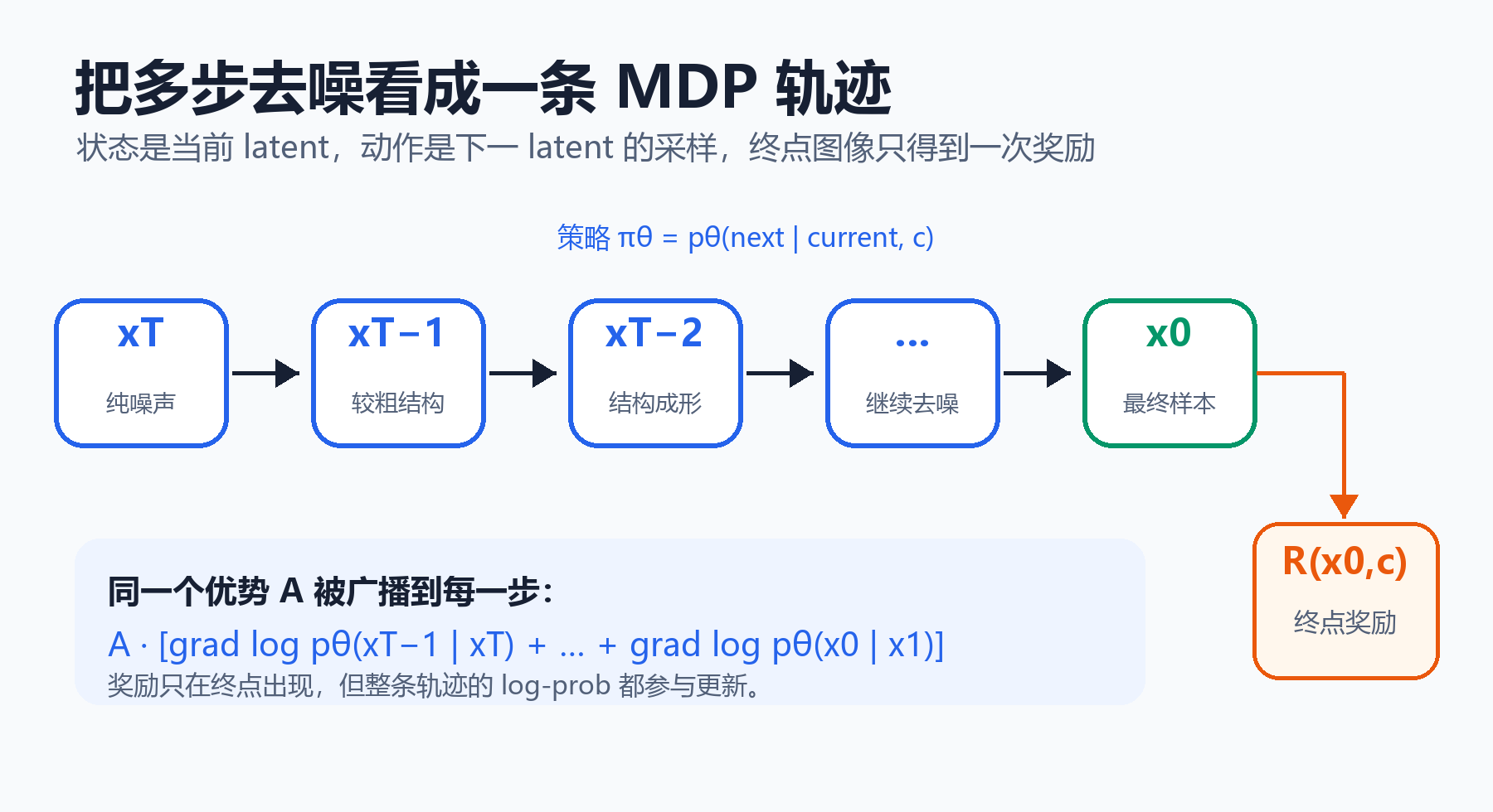
图里有一个必须说准的细节：网络通常输出噪声、velocity 或转移均值的参数，但在 MDP 记号中，“动作”是实际采样出来的 $x_{t-1}$。也就是说，网络参数化动作分布，采样器从这个分布中抽出动作；不要把“网络输出”和“环境中发生的动作”混成一件事。

03. 数学推导

3.1 先把一次随机去噪写成概率分布

为避免被不同预测参数化淹没，先只保留采样器真正需要的形式。对当前 latent $x_t$，模型根据时间步 $t$ 和条件 $c$ 预测噪声，再由调度器算出一个转移均值：

$$\mu_\theta(x_t,t,c).$$

带随机性的 DDIM 步可以统一写成：

$$x_{t-1}=\mu_\theta(x_t,t,c)+\sigma_t z_t,\qquad z_t\sim\mathcal N(0,I).$$

因此条件转移是一个高斯策略：

$$\pi_\theta(a_t\mid s_t)=p_\theta(x_{t-1}\mid x_t,t,c)=\mathcal N\!\left(x_{t-1};\mu_\theta(x_t,t,c),\sigma_t^2 I\right).$$

DDIM 中的随机强度由 ​$\eta$ 控制。训练 DDPO 时通常必须让 ​$\eta>0$，这样被纳入似然目标的随机步骤才有普通高斯密度可用于 log-prob 和重要性比率。注意 $\eta>0$ 仍不保证所有步骤 $\sigma_t>0$：落到干净端的终步可能方差为零，需排除该步或显式采用非零方差，不能直接算高斯 log-prob。若 ​$\eta=0$，转移退化为确定性映射，​$\sigma_t=0$，直接套高斯 log-prob 会除以零；确定性采样仍可用于可微奖励反传，但不能不加处理地套用这套随机策略梯度。

3.2 MDP 的四个元素

把扩散采样改写成 MDP 时，可使用下面的对应关系：

RL 概念	扩散采样中的对象
状态 $s_t$	当前 latent、时间步和条件：​$(x_t,t,c)$
动作 $a_t$	从模型给出的分布中采样下一 latent：​$x_{t-1}$
策略 ​$\pi_\theta$	反向去噪转移 ​$p_\theta(x_{t-1}\mid x_t,t,c)$
奖励	中间步骤通常为 0；解码 ​$x_0$ 后得到 ​$R(x_0,c)$

这里的“环境”几乎没有额外动力学：动作 $x_{t-1}$ 本身就成为下一状态的一部分，时间步从 $t$ 减到 $t-1$。文本编码器、VAE 解码器和奖励模型通常不属于策略参数；真正更新的是 UNet、DiT 或其 LoRA 适配器。

3.3 终点一个分数，为什么每一步都有梯度

给定提示词，一条轨迹记作 ​$\tau=(x_T,x_{T-1},\ldots,x_0)$。因为初始噪声不依赖模型参数，轨迹概率可分解为：

$$p_\theta(\tau\mid c)=p(x_T)\prod_{t=T}^{1}p_\theta(x_{t-1}\mid x_t,t,c).$$

取对数后，乘积变为求和：

$$\log p_\theta(\tau\mid c)=\log p(x_T)+\sum_{t=T}^{1}\log p_\theta(x_{t-1}\mid x_t,t,c).$$

目标是最大化期望终点奖励：

$$J(\theta)=\mathbb E_{c,\tau\sim p_\theta}[R(x_0,c)].$$

应用 likelihood-ratio trick：

$$\nabla_\theta J(\theta)=\mathbb E\!\left[R(x_0,c)\nabla_\theta\log p_\theta(\tau\mid c)\right]=\mathbb E\!\left[R(x_0,c)\sum_{t=T}^{1}\nabla_\theta\log p_\theta(x_{t-1}\mid x_t,t,c)\right].$$

这就是“奖励只在终点，梯度覆盖全轨迹”的来源。实践中会减去不依赖当前动作的基线 $b(c)$，得到优势：

$$A=R(x_0,c)-b(c).$$

减基线不会改变期望梯度，却能显著降低采样方差。若同一个 prompt 一次生成多张图，可以用组内均值和标准差做归一化：

$$A_i=\frac{R_i-\operatorname{mean}(R_{1:G})}{\operatorname{std}(R_{1:G})+\epsilon}.$$

组均值包含自身时，未标准化的中心化 score 估计在独立采样条件下有 $(1-1/G)$ 的缩放；随机标准差还会改变各组权重。因此上面的无偏基线证明不能直接套到组内标准化。它和 GRPO 的“组内相对分数”很相似，不过动作空间从 token 变成了高维 latent 转移。

3.4 每一步的 log-prob 到底怎么算

设动作 $x_{t-1}$ 有 $D$ 个独立高斯坐标、固定方差为 $\sigma_t^2>0$。真实联合 log-prob 必须对坐标求和：

$$\ell_\theta=-\frac{\|x_{t-1}-\mu_\theta\|^2}{2\sigma_t^2}-D\log\sigma_t-\frac D2\log(2\pi).$$

真实逐步联合概率比为 $r_t=\exp(\ell_\theta-\ell_{old})$。DDPO 作者实现 则把逐坐标 log-prob 取平均，即 $\bar\ell=\ell/D$，再计算

$$\bar r_t=\exp(\bar\ell_\theta-\bar\ell_{old})=r_t^{1/D}.$$

这是一种控制高维数值尺度的工程替代比率，不再是严格的联合重要性权重；它也改变了 clip 的尺度。本文一维玩具 $D=1$ 时二者相同，多维复现时必须明确采用哪个约定。下式的 $r_t$ 应按所选约定解释。

PPO 风格的裁剪目标是：

$$L_t(\theta)=\min\!\left(r_t A,\operatorname{clip}(r_t,1-\epsilon,1+\epsilon)A\right).$$

训练代码通常最小化 ​$-L_t$。关键是先按转移计算比率再裁剪，不是先把所有 $r_t$ 相乘成一个轨迹比率。后者会随步数快速积累方差，也让某一步的异常比率拖垮整条样本。

3.5 同一个优势，不代表每一步得到同样的梯度

优势 $A$ 可以广播给每一步，但 score function 不同。对固定方差的高斯策略，有：

$$\nabla_\theta\log p_\theta(x_{t-1}\mid x_t,c)=\frac{x_{t-1}-\mu_\theta}{\sigma_t^2}\nabla_\theta\mu_\theta.$$

时间步的噪声尺度、采样残差、网络 Jacobian 都不同，因此各步的梯度贡献不会相等。终点附近通常对最终结果影响更直接，但并不存在“最后一步天然包办所有学习”的定理；调度器与模型参数化会改变信用在各步之间的分布。

04. 代码实现

下面的玩具过程只有一个可训练标量 ​$\theta$，但保留了 DDPO 的核心结构：8 步高斯去噪、只在终点计算奖励、保存逐步 log-prob、用中心化优势做 REINFORCE，并在最后演示新旧策略的 PPO 比率。

状态转移是：

$$x_{t-1}=0.72x_t+0.18\theta+0.45z_t,\qquad z_t\sim\mathcal N(0,1).$$

终点目标为 1.5，奖励为：

$$R(x_0)=-(x_0-1.5)^2.$$

完整代码见文末。直接运行：

python3 ddpo_minimal.py

真实输出如下：

trajectory_shape= (4096, 9)
transition_log_prob_shape= (4096, 8)
before_terminal_mean= 0.0052
before_reward_mean= -2.6513
after_theta= 2.2677
after_terminal_mean= 1.3577
after_reward_mean= -0.4370
per_step_gradient= [0.0088 0.0085 0.014  0.024  0.0358 0.0435 0.0578 0.0883]
gradient_sample_std_raw_centered= 1.6981 1.3899
ppo_ratio_mean_min_max= 1.0010 0.4051 2.2337
ppo_clip_fraction= 0.3108
history_first= [ 0.     -0.0165 -2.7295]
history_last= [ 2.2677  1.3601 -0.4503]

几个 shape 很重要：4096 条轨迹、每条 8 个转移，所以状态数组有 9 个点，而 log-prob 只有 8 个。训练前 $x_0$ 均值约为 0；40 次更新后移到 1.36，接近目标 1.5，平均奖励从 -2.65 提升到约 -0.44。奖励是负平方误差，所以“更大”意味着更接近 0，而不是数值绝对值更大。

中心化前后，单样本梯度估计的标准差从 1.70 降到 1.39。这只是最简单的 batch baseline；工业实现还会按 prompt 维护统计量，避免一个本来就容易拿高分的 prompt 主导更新。

最后把参数轻微扰动，逐步比率均值仍约为 1，但极端值已经到 0.41 和 2.23，有约 31% 的转移落到裁剪区间之外。这说明“平均比率看起来正常”不足以判断更新是否安全，还要看 clip fraction、KL 和比率分位数。

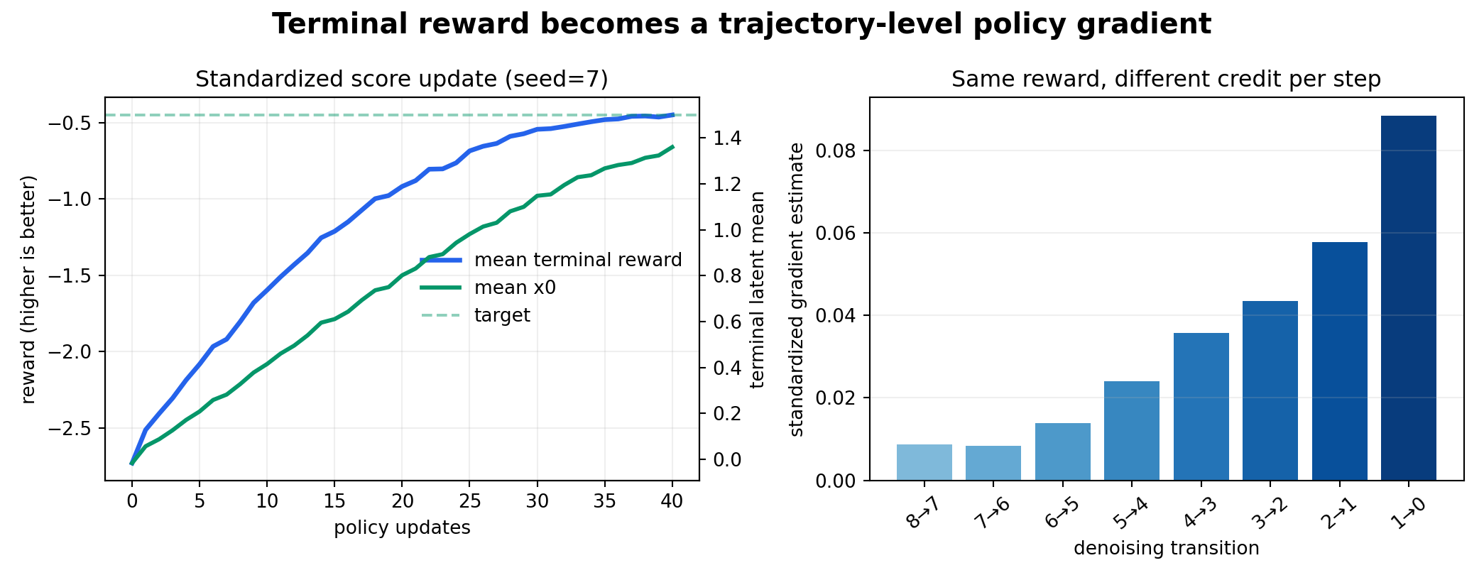
右图里越靠近终点的转移贡献越大，是这个线性玩具过程的收缩系数 0.72 造成的：早期扰动经过多次收缩后影响变小。真实扩散模型不会总呈现这种单调形状，但它直观说明了：即使每一步共享同一个终点优势，信用仍由每一步的局部概率结构决定。

05. 工业级实现对照

截至 2026 年 9 月，DDPO 论文作者维护的参考实现 kvablack/ddpo-pytorch 仍是理解训练循环最直接的代码入口。其 scripts/train.py 和带 log-prob 的 ddim_step_with_logprob 展示了完整数据流：

1. 采样 rollout：从 prompt 和初始噪声出发，保存形状近似为 [batch, steps + 1, C, H, W] 的 latents，以及 [batch, steps] 的旧策略 log-prob。
2. 只给终点打分：将 $x_0$ 经 VAE 解码成图片，用 JPEG 可压缩性、审美分数、目标检测、视觉语言模型或业务规则计算奖励。慢奖励可以并发执行，但返回时必须和样本一一对齐。
3. 构造优势：对全批次奖励标准化，或用 per-prompt statistics tracker 做条件化标准化。同一条轨迹的优势广播到各去噪时间步。
4. 打乱样本与时间步：实现不仅 shuffle 样本，还可对每个样本打乱时间步顺序，降低相邻去噪步相关性对小批次更新的影响。
5. 重算 log-prob：把保存的 $(x_t,x_{t-1},t,c)$ 喂给当前模型，通过 patched DDIM step 得到新策略 log-prob，而不是重新采样一个 $x_{t-1}$。
6. PPO 裁剪更新：计算逐步新旧比率，应用 clipped surrogate loss；通常只训练 LoRA，以降低显存、通信和策略漂移。

这个实现细节解释了为什么训练内存明显大于普通推理：rollout 阶段要保存整条 latent 轨迹和旧 log-prob，更新阶段又要为当前时间步建立反向图。若 rollout batch 为 $B$、去噪步数为 $T$，一轮采样至少处理 $B\times T$ 次 UNet/DiT 前向；若每批 rollout 做 $K$ 个 inner epochs，更新成本还会近似再乘 $K$。梯度累积只改变峰值显存，不会凭空消除总计算量。

早期 Hugging Face TRL 版本曾提供 DDPOTrainer，但当前上游目录与公开 API 已发生重构。读旧教程时应锁定对应版本，不要假设 trl/trainer/ddpo_trainer.py 在最新版仍是稳定入口；本文因此把论文作者仓库作为代码锚点。

从 rollout 到 update 的数据契约

工程里最值得先写清的不是 Trainer 类，而是一条样本在两个阶段之间必须携带什么。rollout 结束后，每条样本至少要保存 prompt 或其编码、全部时间步、从初始噪声到终点的 latents、旧策略逐步 log-prob、最终图片、原始奖励和经过标准化的优势。若使用 classifier-free guidance，还必须固定无条件分支、guidance scale 和文本编码方式；否则更新阶段重算出来的均值并不是采样时那条策略的均值。

update 阶段只取保存的当前 latent 和下一 latent，调用当前模型重算同一个已发生动作的 log-prob。这里绝对不能重新抽噪声：PPO 问的是“新策略对旧动作给出多大概率”，不是“新策略这次随机采到了什么”。这个区别在 token PPO 中很直观——不会在更新时重采一句回答——换成连续 latent 后却很容易藏在调度器接口里。

还应给 rollout 批次分配不可变的 sample id，并把 prompt、随机种子、reward 版本、模型 checkpoint 和 scheduler 配置写进元数据。这样一旦某个 batch 的 ratio 或奖励异常，能够重放出同一条轨迹并定位问题。只记录最后的 PNG 不够，因为不同 latent 轨迹可能解码成肉眼相近的图片，而策略梯度依赖的是当时每一步的概率。

多卡训练时，全局优势标准化也必须基于所有进程聚合后的奖励，而不是每张卡各算各的。否则不同卡的 prompt 难度稍有偏差，就会得到不同的零点和尺度；随后再做梯度平均，相当于混合了多套不一致的目标。相反，若采用 per-prompt 统计器，应明确冷启动策略：某个 prompt 样本太少时回退到全局统计，避免标准差接近零导致优势被放大。

DPOK：为什么还要加 KL

纯奖励最大化很容易把模型推离预训练分布。DPOK（Diffusion Policy Optimization with KL regularization）在在线策略梯度中加入参考模型约束，可抽象为：

$$J_{\text{DPOK}}(\theta)=\mathbb E[R(x_0,c)]-\beta\,D_{\mathrm{KL}}(p_\theta\|p_{\text{ref}}).$$

​$\beta$ 越大，模型越保守；越小，越容易快速追逐奖励，也越容易丢失多样性或出现奖励投机。PPO clipping 约束的是一次更新相对旧策略的变化，reference KL 约束的是长期相对基座模型的漂移，两者作用并不相同。

DRaFT：奖励可微时，可以不走 score function

如果奖励模型对像素可微，且采样器的整条计算图可以保留，就能把梯度从奖励直接穿过 VAE 与采样步骤反传到扩散模型。DRaFT 将这一路线系统化，并提出截断反传等变体来控制内存与梯度不稳定。

两条路线的选择很清楚：

• DDPO / DPOK：奖励可以是完全黑盒，只需要返回标量；代价是策略梯度方差较高，需要大量 on-policy 样本。
• DRaFT 类方法：能利用奖励的路径导数，梯度通常更直接；但奖励必须可微，且跨很多采样步骤保存或重算计算图，显存与稳定性是主要问题。

它们可以共享同一个奖励定义，却不能把“对奖励求导”和“用奖励乘 log-prob”混写成一套推导。

06. 代价与边界

6.1 它省下了什么

• 不需要奖励函数可微，外部 API、人工评分和离散程序都能接入。
• 不需要为每个目标重新制作大规模成对偏好数据；在线采样能探索当前策略真正会生成的区域。
• 能复用 PPO 的裁剪、KL、优势归一化和诊断工具，把更新幅度控制在可观察范围内。

6.2 它付出了什么

• on-policy 成本高：策略一更新，旧 rollout 很快过期；数据复用能力弱于离线偏好优化。
• 终点信用粗糙：所有步骤共享终点优势，方差高；步数越多、latent 越高维，问题越明显。
• 奖励调用可能成为瓶颈：大型 VLM 或人工评分比去噪本身还慢，异步队列与缓存很重要。
• 探索与画质有冲突：增大 DDIM 的 ​$\eta$ 有利于随机策略探索，却可能改变原有采样质量与分布。
• 奖励投机不会自动消失：OCR 奖励可能鼓励巨大文字，审美分数可能压低多样性，检测器奖励可能诱导模型画出分类器偏爱的纹理。

6.3 上线前至少记录这些指标

不要只看 mean reward。最低限度还应记录：

• 奖励均值、标准差和分位数，按 prompt 类别拆分；
• 新旧策略的 approximate KL、ratio 分位数与 clip fraction；
• 每个时间步的 loss、KL 或梯度范数，检查是否只剩少数步在学习；
• 多样性指标和基础画质指标，防止奖励提高但模式坍缩；
• 人工盲评或独立奖励模型的 holdout 分数，防止只攻破训练用 reward；
• 无效图片、NaN、全黑/过曝和安全过滤命中率。

如果奖励模型本身正在更新，还要给 reward 版本打快照。否则同一条训练曲线纵轴含义会变化，前后 reward 数字不可直接比较。

6.4 奖励怎么配，往往比优化器更重要

真实系统几乎不会只用一个分数。以文字生成图片为例，可以同时有提示词一致性、OCR 正确率、审美、人体结构和安全性五类信号。最直接的做法是加权求和：

$$R=w_{\text{prompt}}R_{\text{prompt}}+w_{\text{ocr}}R_{\text{ocr}}+w_{\text{aesthetic}}R_{\text{aesthetic}}-w_{\text{safety}}C_{\text{safety}}.$$

但“都放进来”不等于问题解决了。不同奖励的量纲与波动范围可能差几个数量级：OCR 是 0 或 1，审美模型可能落在 1 到 10，安全惩罚可能只有极少数样本非零。若不先校准，权重看似相近，实际梯度却会被方差最大的那一项占满。稳妥做法是先在固定基座模型上采一批校准集，观察每项分布，再做裁剪、标准化或分位数映射；训练期间同时画出每个子奖励，不能只保存加权总分。

还要区分“软目标”和“硬约束”。图片里文字少一个字，通常是可连续改进的软目标；生成违法内容则不应靠一个可被其他高分抵消的负权重处理。硬约束更适合在采样前后用过滤器、拒绝策略或拉格朗日约束单独处理。否则模型可能发现：只要审美分足够高，安全惩罚也值得承受。

多目标之间还会发生真实冲突。把 OCR 权重拉高，模型可能把文字做得巨大而破坏构图；只奖励检测器置信度，可能得到边缘锐利但不自然的目标。应当用 Pareto 视角看结果：同一批 checkpoints 同时比较各子目标和人工偏好，选择没有被某一维明显支配的方案，而不是盯着一条总 reward 曲线挑最高点。

6.5 三个能快速定位实现错误的不变量

第一，rollout 保存的状态数必须比转移 log-prob 数多 1；若二者相等，通常漏了初始噪声或终点 latent。第二，当新旧模型参数完全相同时，逐步 ratio 应非常接近 1，approximate KL 应接近 0；否则多半是调度器、CFG 分支、时间步索引或 log-prob 归约维度不一致。第三，打乱 batch 顺序不应改变同一个样本的 reward、prompt、latents 与 log-prob 对齐关系。异步奖励最容易在这里悄悄错位：训练仍会运行，均值甚至会上升，但模型学到的是别人的分数。

调试时先用一个可以解析求解的低维过程，就像本文代码；确认梯度方向、ratio 和 baseline 都符合预期，再接入大模型。直接在多卡图像训练里找符号错误，通常会把昂贵计算浪费在最便宜的 bug 上。

这些不变量也适合写进自动化测试：用固定随机种子的十几条轨迹做快速回归，每次升级 diffusers、调度器或混合精度设置后先跑它，再启动昂贵的正式训练。

07. 经典论文脉络

1. Training Diffusion Models with Reinforcement Learning / DDPO（arXiv:2305.13301）把扩散去噪正式改写为多步决策过程，给出基于 likelihood ratio 的 DDPO，并展示了不可微奖励下的微调能力。它奠定了“去噪轨迹就是策略轨迹”的主框架。
2. DPOK: Reinforcement Learning for Fine-tuning Text-to-Image Diffusion Models（arXiv:2305.16381）把在线策略梯度与 KL 正则结合，强调奖励提升和预训练分布保持之间的平衡。
3. DRaFT: Directly Fine-tuning Diffusion Models on Differentiable Rewards（arXiv:2309.17400）转向可微奖励，通过采样链直接反传，并研究 full、截断和低方差版本，形成与 DDPO 互补的路线。
4. Reward-Directed Conditional Diffusion（arXiv:2307.07055）从 reward-conditioned / reward-directed 角度研究如何把黑盒目标引入扩散生成，说明“训练一个条件生成器”和“在线策略优化”是相关但不同的解法。
5. Diffusion Models for Reinforcement Learning: A Survey（arXiv:2311.01223）覆盖的是更宽的交叉方向：既包括用 RL 对齐扩散生成，也包括把扩散模型当作策略或规划器。阅读时要先辨认“RL 优化 diffusion”还是“diffusion 服务 RL”。

论文名称很像时，先看梯度从哪里来：若公式里是 $R\nabla\log p_\theta$，属于 score-function 策略梯度；若是 ​$\nabla_{x_0}R$ 沿采样链反传，则属于可微奖励路线；若训练数据是静态偏好对，通常又是离线偏好优化问题。

08. 常见误解

误解 1：模型预测的噪声就是 RL 动作

噪声预测是策略的参数化中间量。DDPO 的动作通常记为实际采样出的下一 latent $x_{t-1}$，策略概率才是 ​$p_\theta(x_{t-1}\mid x_t,c)$。只有这样，保存动作、重算 log-prob 和构造新旧比率才是一致的。

误解 2：奖励在最后，所以只有最后一步能更新

轨迹 log-prob 是逐步 log-prob 的和。终点奖励乘的是整条和，因此每个去噪转移都有 score-function 梯度。最后一步可能贡献较大，但不是唯一有梯度的一步。

误解 3：确定性 DDIM 也能原样计算 DDPO log-prob

​$\eta=0$ 时 ​$\sigma_t=0$，普通高斯 log-prob 不再成立。要么使用非零随机性，要么换成适合确定性路径的可微反传或其他估计器，不能简单给分母加一个 epsilon 就宣称理论等价。

误解 4：把所有逐步比率相乘，才是最“严格”的 PPO

轨迹比率在长链上方差巨大。DDPO 实践通常按去噪转移计算和裁剪 ratio；这是一种稳定的 surrogate，而不是把一个 50 步连乘数硬塞进普通 PPO 公式。

误解 5：同一奖励广播到每一步，所以每步学到的一样

优势相同，不等于 score function 相同。噪声方差、预测残差、网络敏感度和调度器权重都随时间步变化，逐步梯度自然不同。

误解 6：奖励不可微就无法优化扩散模型

DDPO 只需要采样结果和标量奖励，不需要奖励梯度。不可微带来的问题是估计方差和样本成本，而不是“没有任何梯度”。

误解 7：训练 reward 上升就代表模型全面变好

模型可能只学会利用 reward 的盲点。必须同时看独立评估、人工盲评、多样性、prompt 遵循和安全指标；最好用不同架构的 holdout reward 检查泛化。

09. 动手验证：四个改动看懂算法

文末代码只依赖 NumPy，建议依次改四个参数，每次固定随机种子并比较输出。

实验 A：把 steps 从 8 改为 16

预期状态 shape 从 (4096, 9) 变成 (4096, 17)，log-prob shape 从 (4096, 8) 变成 (4096, 16)。更长轨迹会增加梯度求和项；在不调整学习率与归一化时，训练波动通常更明显。

实验 B：把 noise_std 从 0.45 降到 0.10

探索减弱，采样更集中；但 score function 含 ​$1/\sigma^2$，数值会更尖锐。过小噪声并不等于更稳定，极限到 0 反而失去这套高斯策略梯度的基础。

实验 C：删掉优势中心化

把 advantage = (reward - reward.mean()) / ... 改成直接使用 reward。gradient_sample_std_raw_centered 的第二个值会失去优势，训练曲线更抖。这个实验直观看到 baseline 改变方差而不改变目标最优点。

实验 D：增大新旧参数差

在 PPO 诊断部分增大 new_theta - old_theta。你会看到 ratio_min/max 更极端，clip_fraction 上升。工程上这对应学习率过大、inner epochs 过多或 KL 约束过弱。

进一步可把终点奖励改成离散黑盒：例如 reward = (abs(x0-target) < 0.25)。代码仍能训练，但由于奖励更稀疏，往往需要更大 batch、分层采样或更好的 baseline。这正是从玩具例子走向 OCR 成功率、目标检测命中和人工反馈时遇到的现实问题。

10. 延伸阅读

这篇位于“对齐与强化学习”路径的第三段：

1. 策略梯度与 PPO 基础：理解 advantage、ratio、clipping 和 KL；
2. 从 DPO 到 GRPO：去掉价值网络：理解组内相对优势；
3. 本文 DiffusionRL：把 token 轨迹换成 latent 去噪轨迹；
4. 视频生成中的强化学习与奖励模型：在去噪信用之外，再处理画质、运动与指令遵循的多目标奖励。

如果 DDIM 还不熟，先记住本文真正依赖的最小事实：它把 $x_t$ 和网络预测组合成下一步均值，并可用 ​$\eta$ 注入高斯随机性。从 DDIM 到高阶采样器 已展开采样公式、ODE/SDE 视角与高阶求解器。

最后用一句话收束：

DiffusionRL 不是把一个 PPO 套在图片外面，而是把每次去噪转移变成可计概率的动作，再让终点奖励沿整条轨迹分配信用。

附录：完整代码

09 节用到的脚本全文如下（ddpo_minimal.py、make_figures.py）。复制到本地存成同名文件，按各脚本开头的依赖说明准备环境后即可运行。

ddpo_minimal.py

"""NumPy-only toy DDPO: treat iterative denoising as a stochastic policy.

This is an algebra demo, not an image generator.  A scalar latent follows a
short Gaussian reverse process.  One parameter shifts every denoising mean,
and a terminal reward teaches the process to end near a target value.
"""

from dataclasses import dataclass

import numpy as np


@dataclass(frozen=True)
class ToyConfig:
    steps: int = 8
    batch_size: int = 4096
    contraction: float = 0.72
    action_scale: float = 0.18
    noise_std: float = 0.45
    target: float = 1.5


def gaussian_log_prob(value, mean, std):
    """Elementwise log N(value; mean, std^2)."""
    return -0.5 * ((value - mean) / std) ** 2 - np.log(std * np.sqrt(2.0 * np.pi))


def rollout(theta, cfg, rng):
    """Sample x_T -> ... -> x_0 and retain every transition.

    Array index 0 stores x_T; index cfg.steps stores x_0.  The transition
    mean is mu_theta = contraction * x_t + action_scale * theta.
    """
    latents = np.empty((cfg.batch_size, cfg.steps + 1), dtype=np.float64)
    means = np.empty((cfg.batch_size, cfg.steps), dtype=np.float64)
    log_probs = np.empty((cfg.batch_size, cfg.steps), dtype=np.float64)
    latents[:, 0] = rng.normal(size=cfg.batch_size)

    for j in range(cfg.steps):
        mean = cfg.contraction * latents[:, j] + cfg.action_scale * theta
        next_latent = mean + cfg.noise_std * rng.normal(size=cfg.batch_size)
        latents[:, j + 1] = next_latent
        means[:, j] = mean
        log_probs[:, j] = gaussian_log_prob(next_latent, mean, cfg.noise_std)

    terminal = latents[:, -1]
    rewards = -(terminal - cfg.target) ** 2
    return latents, means, log_probs, rewards


def score_function(latents, means, cfg):
    """d log pi_theta(x_{t-1}|x_t) / d theta for every transition."""
    residual = latents[:, 1:] - means
    return residual * cfg.action_scale / (cfg.noise_std**2)


def policy_gradient(rewards, per_step_scores):
    """REINFORCE with a batch baseline; terminal advantage is broadcast to T steps."""
    centered = rewards - rewards.mean()
    advantages = centered / (rewards.std() + 1e-8)
    trajectory_scores = per_step_scores.sum(axis=1)
    gradient = np.mean(advantages * trajectory_scores)
    per_step_gradient = np.mean(advantages[:, None] * per_step_scores, axis=0)
    return gradient, per_step_gradient, advantages


def evaluate(theta, cfg, seed):
    rng = np.random.default_rng(seed)
    latents, means, log_probs, rewards = rollout(theta, cfg, rng)
    return {
        "terminal_mean": float(latents[:, -1].mean()),
        "reward_mean": float(rewards.mean()),
        "latents": latents,
        "means": means,
        "log_probs": log_probs,
        "rewards": rewards,
    }


def train(cfg, updates=40, learning_rate=0.08, seed=7):
    theta = 0.0
    history = []
    rng = np.random.default_rng(seed)

    for update in range(updates + 1):
        latents, means, _, rewards = rollout(theta, cfg, rng)
        scores = score_function(latents, means, cfg)
        gradient, per_step_gradient, advantages = policy_gradient(rewards, scores)
        history.append((update, theta, latents[:, -1].mean(), rewards.mean(), gradient))
        if update < updates:
            theta += learning_rate * gradient

    return theta, np.asarray(history), per_step_gradient, advantages, scores, rewards


def ppo_diagnostics(theta_old, theta_new, cfg, seed=123, clip_range=0.2):
    """Re-evaluate old transitions under a candidate new policy."""
    rng = np.random.default_rng(seed)
    latents, old_means, old_log_probs, rewards = rollout(theta_old, cfg, rng)
    new_means = cfg.contraction * latents[:, :-1] + cfg.action_scale * theta_new
    new_log_probs = gaussian_log_prob(latents[:, 1:], new_means, cfg.noise_std)
    ratios = np.exp(new_log_probs - old_log_probs)
    clipped = np.abs(ratios - 1.0) > clip_range
    return rewards, ratios, clipped


if __name__ == "__main__":
    np.set_printoptions(precision=6, suppress=True)
    cfg = ToyConfig()

    before = evaluate(theta=0.0, cfg=cfg, seed=2026)
    theta, history, per_step_gradient, advantages, scores, rewards = train(cfg)
    after = evaluate(theta=theta, cfg=cfg, seed=2026)

    raw_gradient_samples = rewards * scores.sum(axis=1)
    centered_gradient_samples = (rewards - rewards.mean()) * scores.sum(axis=1)
    ppo_rewards, ratios, clipped = ppo_diagnostics(
        theta_old=0.0, theta_new=0.5, cfg=cfg
    )

    print("trajectory_shape=", before["latents"].shape)
    print("transition_log_prob_shape=", before["log_probs"].shape)
    print("before_terminal_mean=", f"{before['terminal_mean']:.4f}")
    print("before_reward_mean=", f"{before['reward_mean']:.4f}")
    print("after_theta=", f"{theta:.4f}")
    print("after_terminal_mean=", f"{after['terminal_mean']:.4f}")
    print("after_reward_mean=", f"{after['reward_mean']:.4f}")
    print("per_step_gradient=", np.round(per_step_gradient, 4))
    print(
        "gradient_sample_std_raw_centered=",
        f"{raw_gradient_samples.std():.4f}",
        f"{centered_gradient_samples.std():.4f}",
    )
    print(
        "ppo_ratio_mean_min_max=",
        f"{ratios.mean():.4f}",
        f"{ratios.min():.4f}",
        f"{ratios.max():.4f}",
    )
    print("ppo_clip_fraction=", f"{clipped.mean():.4f}")
    print("history_first=", np.round(history[0, 1:4], 4))
    print("history_last=", np.round(history[-1, 1:4], 4))

    assert before["latents"].shape == (cfg.batch_size, cfg.steps + 1)
    assert before["log_probs"].shape == (cfg.batch_size, cfg.steps)
    assert after["reward_mean"] > before["reward_mean"]
    assert abs(after["terminal_mean"] - cfg.target) < abs(before["terminal_mean"] - cfg.target)
    assert np.all(np.isfinite(ratios))

make_figures.py

"""Generate the explanatory figures for the DiffusionRL article.

Requires NumPy, Matplotlib and Pillow.  The numerical chart reuses the exact
toy process from ddpo_minimal.py so the article and figure cannot drift apart.
"""

from pathlib import Path

import matplotlib

matplotlib.use("Agg")
import matplotlib.pyplot as plt
import numpy as np
from PIL import Image, ImageDraw, ImageFont

from ddpo_minimal import ToyConfig, train


OUT = Path(__file__).resolve().parents[1] / "figures"
OUT.mkdir(exist_ok=True)


def _font(size, bold=False):
    candidates = (
        "/System/Library/Fonts/PingFang.ttc",
        "/System/Library/Fonts/Hiragino Sans GB.ttc",
        "/usr/share/fonts/opentype/noto/NotoSansCJK-Bold.ttc" if bold else
        "/usr/share/fonts/opentype/noto/NotoSansCJK-Regular.ttc",
    )
    for path in candidates:
        try:
            return ImageFont.truetype(path, size)
        except OSError:
            pass
    raise RuntimeError("请安装中文字体后再生成 DiffusionRL 示意图")


def trajectory_mdp():
    image = Image.new("RGB", (1800, 980), "#f8fafc")
    draw = ImageDraw.Draw(image)
    ink, blue, green, orange, muted = "#172033", "#2563eb", "#059669", "#ea580c", "#526078"

    draw.text((90, 55), "把多步去噪看成一条 MDP 轨迹", font=_font(70, True), fill=ink)
    draw.text((92, 150), "状态是当前 latent，动作是下一 latent 的采样，终点图像只得到一次奖励", font=_font(38), fill=muted)
    draw.text((900, 285), "策略 πθ = pθ(next | current, c)", font=_font(32), fill=blue, anchor="mm")

    xs = [170, 480, 790, 1100, 1410]
    labels = ["xT", "xT−1", "xT−2", "…", "x₀"]
    subtitles = ["纯噪声", "较粗结构", "结构成形", "继续去噪", "最终样本"]
    for i, (x, label, subtitle) in enumerate(zip(xs, labels, subtitles)):
        color = blue if i < len(xs) - 1 else green
        draw.rounded_rectangle((x - 105, 360, x + 105, 540), radius=36, fill="#ffffff", outline=color, width=6)
        draw.text((x, 400), label, font=_font(46, True), fill=color, anchor="mm")
        draw.text((x, 485), subtitle, font=_font(28), fill=muted, anchor="mm")
        if i < len(xs) - 1:
            draw.line((x + 110, 450, xs[i + 1] - 120, 450), fill=ink, width=5)
            draw.polygon(
                [(xs[i + 1] - 120, 450), (xs[i + 1] - 148, 433), (xs[i + 1] - 148, 467)],
                fill=ink,
            )

    draw.line((1515, 450, 1650, 450), fill=orange, width=5)
    draw.polygon([(1650, 450), (1622, 433), (1622, 467)], fill=orange)
    draw.rounded_rectangle((1510, 630, 1735, 820), radius=32, fill="#fff7ed", outline=orange, width=5)
    draw.text((1622, 675), "R(x₀,c)", font=_font(44, True), fill=orange, anchor="mm")
    draw.text((1622, 750), "终点奖励", font=_font(31), fill=muted, anchor="mm")
    draw.line((1620, 545, 1620, 625), fill=orange, width=5)
    draw.polygon([(1620, 625), (1603, 597), (1637, 597)], fill=orange)

    draw.rounded_rectangle((90, 650, 1380, 850), radius=30, fill="#eef4ff")
    draw.text((130, 685), "同一个优势 A 被广播到每一步：", font=_font(39, True), fill=ink)
    draw.text((130, 750), "A · [grad log pθ(xT−1 | xT) + … + grad log pθ(x₀ | x₁)]", font=_font(39), fill=blue)
    draw.text((130, 805), "奖励只在终点出现，但整条轨迹的 log-prob 都参与更新。", font=_font(31), fill=muted)

    image.save(OUT / "diffusion_rl_mdp.png", optimize=True)


def cover():
    image = Image.new("RGB", (1280, 720), "#081225")
    draw = ImageDraw.Draw(image)

    # A denoising trajectory that gradually changes from noise-like dots into a
    # clean latent.  Keeping this code-native makes the cover deterministic.
    rng = np.random.default_rng(7)
    stages = [190, 400, 610, 820, 1030]
    palette = ["#60a5fa", "#38bdf8", "#2dd4bf", "#34d399", "#f59e0b"]
    for i, x in enumerate(stages):
        radius = 62
        draw.ellipse((x - radius, 258 - radius, x + radius, 258 + radius), outline=palette[i], width=5)
        spread = 47 - i * 7
        for _ in range(38 - i * 4):
            px = x + int(rng.normal(0, spread))
            py = 258 + int(rng.normal(0, spread))
            dot = 2 + i
            draw.ellipse((px - dot, py - dot, px + dot, py + dot), fill=palette[i])
        if i < len(stages) - 1:
            draw.line((x + 72, 258, stages[i + 1] - 75, 258), fill="#94a3b8", width=4)
            draw.polygon(
                [(stages[i + 1] - 75, 258), (stages[i + 1] - 96, 246), (stages[i + 1] - 96, 270)],
                fill="#94a3b8",
            )

    draw.rounded_rectangle((1068, 190, 1222, 326), radius=26, fill="#431407", outline="#f59e0b", width=4)
    draw.text((1145, 258), "+R", font=_font(48, True), fill="#fbbf24", anchor="mm")
    draw.text((92, 415), "把 RL 用到扩散模型上", font=_font(64, True), fill="#f8fafc")
    draw.text((96, 507), "DiffusionRL · DDPO · 去噪轨迹 · 信用分配", font=_font(34), fill="#93c5fd")
    draw.rounded_rectangle((94, 603, 426, 659), radius=25, fill="#1d4ed8")
    draw.text((260, 631), "AIGC 基本功", font=_font(28, True), fill="#ffffff", anchor="mm")
    image.save(OUT / "wechat_cover_diffusion_rl.png", optimize=True)


def training_and_credit():
    cfg = ToyConfig()
    _, history, per_step_gradient, _, _, _ = train(cfg)
    updates = history[:, 0]

    fig, axes = plt.subplots(1, 2, figsize=(11, 4.3))
    ax = axes[0]
    ax.plot(updates, history[:, 3], color="#2563eb", linewidth=2.5, label="mean terminal reward")
    ax.set_xlabel("policy updates")
    ax.set_ylabel("reward (higher is better)")
    ax.grid(alpha=0.2)
    ax2 = ax.twinx()
    ax2.plot(updates, history[:, 2], color="#059669", linewidth=2.2, label="mean x0")
    ax2.axhline(cfg.target, color="#059669", linestyle="--", alpha=0.45, label="target")
    ax2.set_ylabel("terminal latent mean")
    lines = ax.get_lines() + ax2.get_lines()
    ax.legend(lines, [line.get_label() for line in lines], frameon=False, loc="center right")
    ax.set_title("Toy DDPO learns from terminal reward")

    ax = axes[1]
    steps = np.arange(cfg.steps)
    ax.bar(steps, per_step_gradient, color=plt.cm.Blues(np.linspace(0.45, 0.95, cfg.steps)))
    ax.set_xticks(steps, [f"{cfg.steps-i}→{cfg.steps-i-1}" for i in steps], rotation=40)
    ax.set_xlabel("denoising transition")
    ax.set_ylabel("estimated gradient contribution")
    ax.grid(axis="y", alpha=0.2)
    ax.set_title("Same reward, different credit per step")

    fig.suptitle("Terminal reward becomes a trajectory-level policy gradient", fontsize=15, weight="bold")
    fig.tight_layout()
    fig.savefig(OUT / "diffusion_rl_training_credit.png", dpi=190)
    plt.close(fig)


if __name__ == "__main__":
    trajectory_mdp()
    training_and_credit()
    cover()
    for name in (
        "diffusion_rl_mdp.png",
        "diffusion_rl_training_credit.png",
        "wechat_cover_diffusion_rl.png",
    ):
        print(OUT / name)

---

---

更多 AIGC 论文解读，关注微信公众号「人工智能炼丹君」

每日更新 · 论文精选 · 深度解读 · 技术脉络

微信搜索 人工智能炼丹君 或扫描下方二维码关注