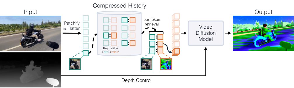
Figure 2 : Correspondence-based video translation. The memory is populated with input-output correspondence pairs from previous generations. To support the consistent translation of the next block of frames, we first retrieve from memory the output patches whose corresponding input is most similar to the current. These output patches, together with the normal input signal, is the input to our video diffusion model. Based on the new induced input-output pairs, we write to memory only those that are sufficiently different from existing.
Figure 3 : Qualitative comparisons. We show two frames sampled far apart in time for three example videos (left and right). Bidirectional methods (VACE 1.3B) and Autoregressive distillation methods produce high-quality individual frames but fail to maintain object identity over long durations. Adding our correspondence mechanism preserves consistent appearance throughout the video.
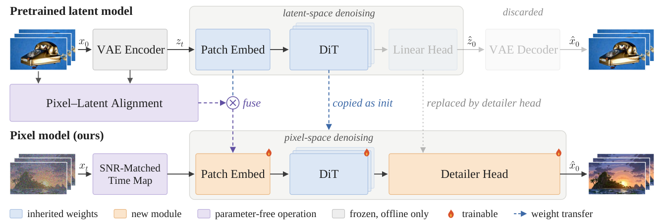
Figure 2 : Lifting a pretrained latent video DiT to pixel space. Top: the pretrained latent model. A linear pixel-latent alignment, fitted offline, is fused with the pretrained patch embedding to obtain a pixel patch embedding. Bottom: PixVid. A timestep calibration rescales noisy pixel input to the signal-to-noise ratio the pretrained DiT was trained on. The DiT is initialized from the latent model, and a convolutional detailer head replaces the linear head and VAE decoder to predict the clean video directly.
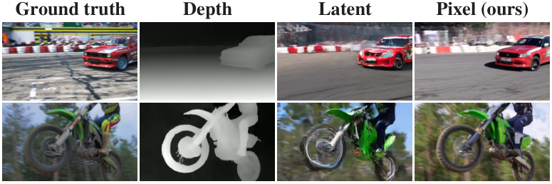
Figure 5 : Depth-conditioned Editing. Our pixel model enables precise video editing under high motion, while the temporally compressed latent model morphs and blurs fast-moving objects.
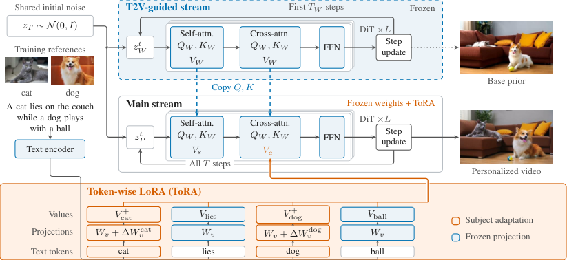
Figure 2 : Overall framework of TokenStream. Subject adapters are learned independently and applied only to their text-token spans in the value projection. The frozen T2V-guided stream transfers Q , K Q,K attention features during the first T W T_{W} denoising steps; the personalized stream retains its values and continues for all T T steps. Each model evaluation traverses L L self-attention–cross-attention–FFN blocks. Both streams share frozen weights but incur additional guidance computation.
实验效果:在作者的 Multi-DB(30 个主体、122 条提示)1.3B 设定中,身份保持 IP 从 DreamBooth 的 0.422 到 0.467,文本对齐 TA 从 0.652 到 0.688;两项分数越高越好。这是指定基准和对照,并非全表最优:Phantom 的 IP 为 0.510。
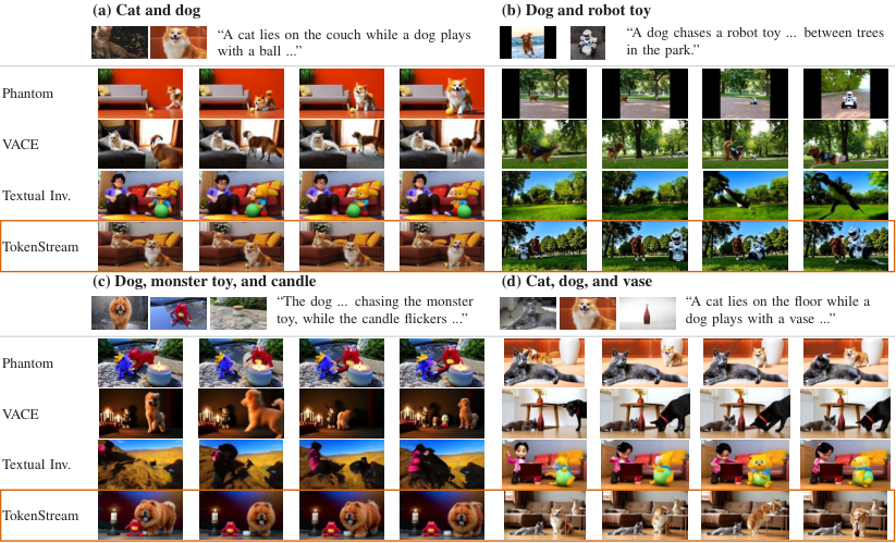
Figure 4 : Qualitative comparisons on Multi-DB. Selected examples illustrate subject binding and prompt-conditioned composition. They do not establish reliable articulated motion or success on every scene; omission, identity mixing, and same-class failures are shown in the supplement.
批判点评:冻结引导流仍带来额外计算;主体数量增大时漏主体和混身份更明显。原文 14B OpenS2V-Eval 中本法 IP 0.482,低于 MAGREF 的 0.567,不能泛称在所有基准胜出。
4. TRACE:视频升分辨率快2.0至2.9倍
TRACE: Trajectory Synchronization for Training-Free Resolution Extension in Video Generation | 上海交通大学;华为;西北工业大学;西安电子科技大学 | arXiv:2611.15983
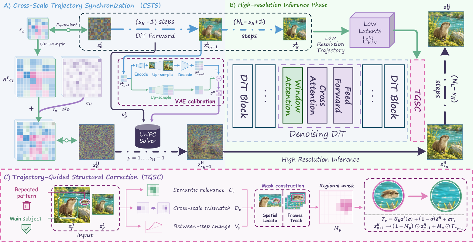
Figure 3 : Overview of TRACE . The low-resolution trajectory ( Low ) provides scene references for the high-resolution trajectory ( High ). (A) CSTS couples their initial noise and computes early High updates from Low’s predictions, avoiding high-resolution model inferences. (B) Window attention computes high-resolution model predictions. (C) TGSC uses semantic relevance, cross-scale mismatch and between-step change to select suspected duplicated subjects. It corrects those latent regions and the corresponding solver history.
Figure 6 : Visual comparison of direct inference and training-free resolution-extension methods at × 1088 1920\!\times\!1088 on Wan2.1. Each result pairs two adjacent frames with a detail crop, highlighting wood texture, building facades, and local structure.
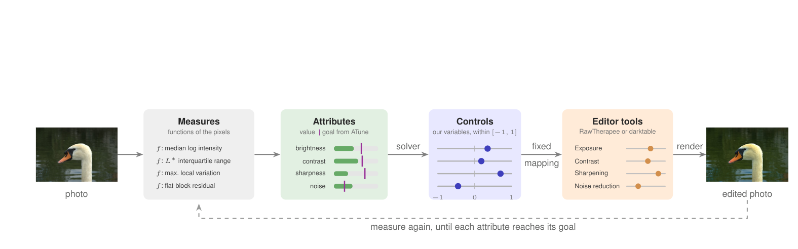
Figure 6 : Attribute, measure, control and tool. An attribute is a quality of the photograph, such as sharpness; its measure is the function that computes it from the pixels ( Appendix A ). ATune sets a goal for each attribute. Each attribute has one control , our own variable within [ − 1 , 1 ] [-1,1] ; a fixed mapping turns it into settings of the editor’s tools ( Tab. 8 ).
实验效果:157 位评审做出 9253 次成对选择:同一编辑器条件下,相对 GPT-6 Astra 的编辑,人类有 54.3% 选择 ATune;相对 Claude Opus 5 为 50.5%。对在各自专家数据集训练的监督修图器,ATune 获选 46.3%,并未获多数偏好。
Figure 2 : Three example edits. We score every FiveK and PPR10K photograph by how much the nine judges prefer our edit to Claude’s, and show one photograph the judges clearly give to ours (top), a typical one (middle) and one they clearly give to Claude (bottom). The badge on each edit counts the judges that score it above the other. Below each image: the boxed region enlarged.
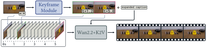
Figure 2. Overview of the proposed method. We design a keyframe module which reasons about the physical evolution of a given scene and produces keyframes with timestamps and an expanded caption. These are then used as the conditioning signal for Wan2.2, resulting in videos with more accurate physical plausibility.
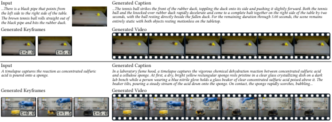
Figure 5. Qualitative results from our approach. The top row shows an example from Physics-IQ Verified and the bottom row an example from PhyGenBench. These results highlight the diverse placement of keyframes in different videos, and the physical quality of the resulting generated videos.
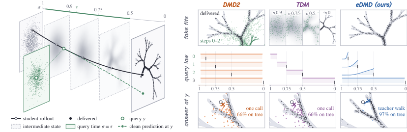
本文贡献:eDMD(Endpoint Distribution Matching Distillation)只用学生最终图像训练共享假模型,再将其端点参照用于各去噪步;另加精确教师短轨迹与校准的中间查询密度。DMD 是分布匹配蒸馏,学生是缩短采样步数的生成器。
Figure 2 : Overview of eDMD on a 2D tree-structured toy distribution (gray). Left: a 4-step student denoises from noise ( σ = 1 \sigma=1 ) to its final output ( σ = 0 \sigma=0 , “delivered”); each update noises one step’s prediction to a level τ \tau (green bar: its range) and compares the teacher and the fake model at the resulting query \mathbf{y} . Right: compared with DMD2 and TDM, eDMD trains the fake model on final outputs only (top), draws the queries of intermediate steps from a calibrated density (middle; ticks: the level each step denoises to), and answers low-noise queries with a multi-step teacher instead of a single prediction (bottom; percentages: answers on the tree).
Figure 4 : Qualitative results on FLUX.2-klein-4B. Leftmost: teacher (50 steps, w = 4 w=4 ); others: 4-step students at the checkpoints of Tab. 1 ; shared prompt and noise per row. Best viewed zoomed in: on fine structures such as fur, hair, and grass, eDMD preserves richer details and fewer artifacts, yielding more natural textures than existing methods.
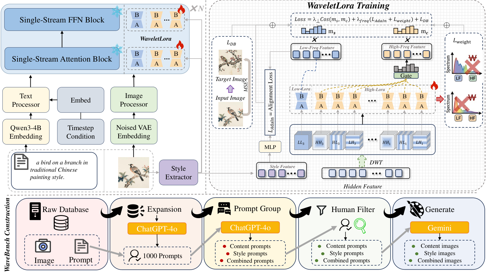
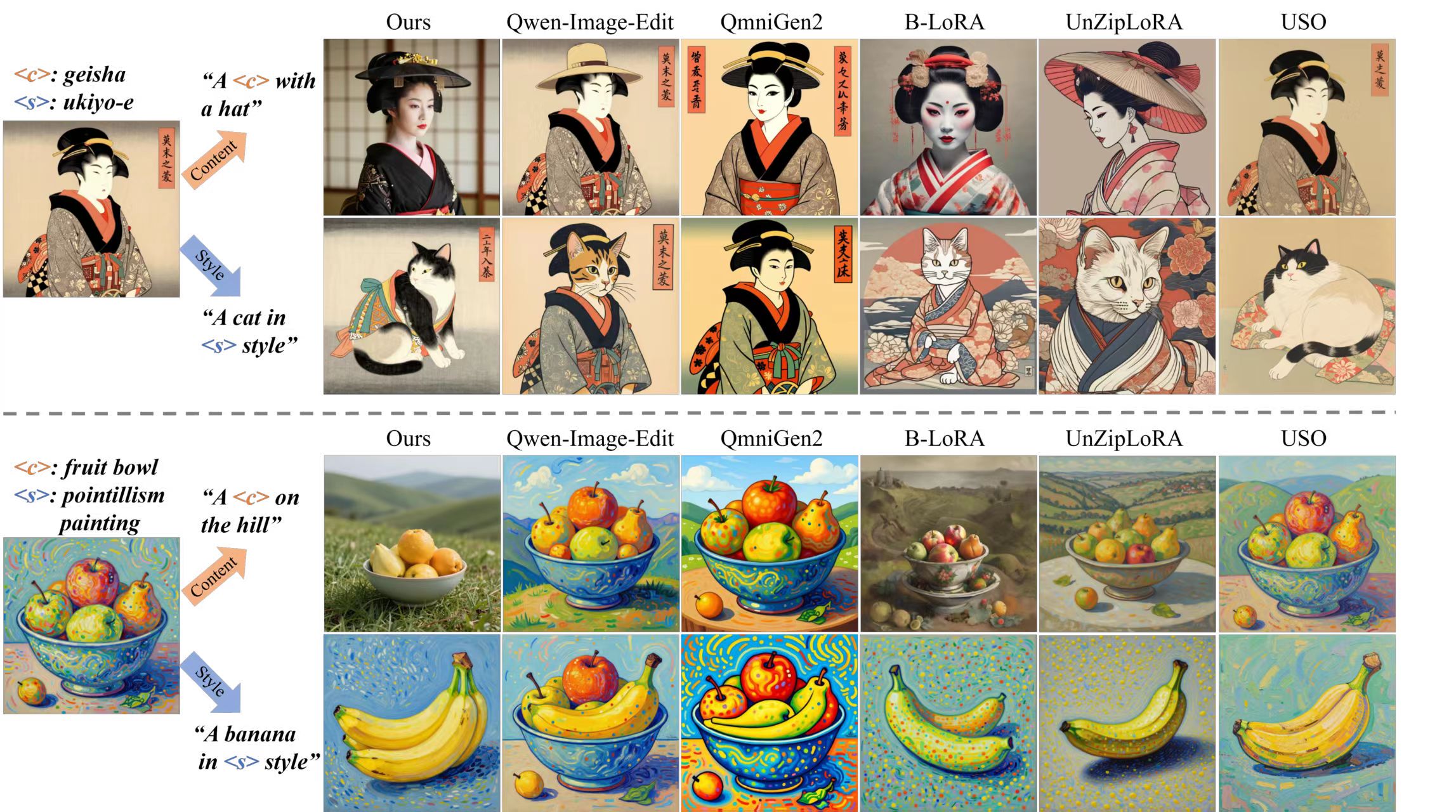
Figure 2 : Overview of WaveletLoRA and WaveBench. (Top) Given a reference image, a two-level DWT decomposes the image into one low-frequency subband and multiple high-frequency subbands. The low-frequency branch learns global appearance attributes for style modeling, while the high-frequency branches preserve multi-scale structural details for content representation. An adaptive aggregation MoE module fuses high-frequency representations into a unified content LoRA, followed by frequency-domain disentanglement supervision and AdaIN-based style alignment. (Bottom) Construction pipeline of WaveBench, including prompt generation, manual verification, and reference image synthesis.
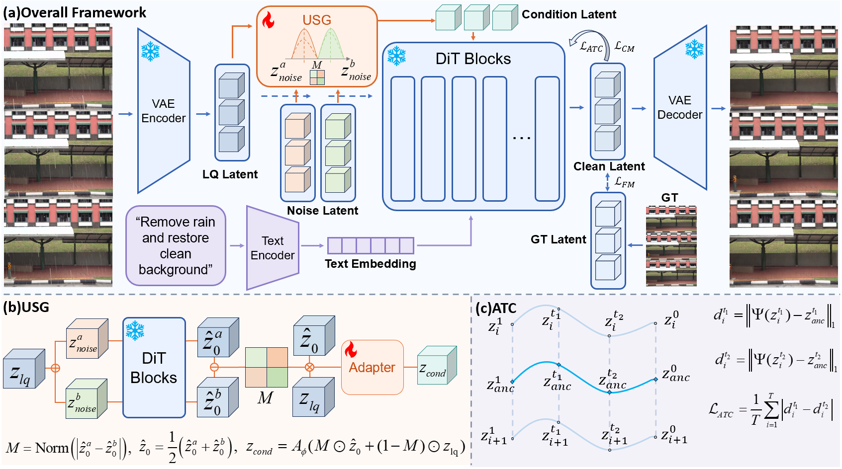
Fig. 2: Overall architecture of the proposed SGVD for video deraining. The rainy video is first encoded into the latent space by a frozen VAE encoder. The Uncertainty-Guided Selective Generation (USG) module estimates a spatial uncertainty map from the discrepancy between dual-noise clean latent predictions, and adaptively combines the generative latent with the fidelity-preserving LQ latent. The resulting conditional latent is injected into the frozen DiT backbone through a lightweight trainable adapter. Meanwhile, Anchor-Guided Trajectory Consistency (ATC) regularizes each frame's distance to a shared five-frame anchor across trajectory states, promoting temporal coherence without evaluating this training loss at inference.
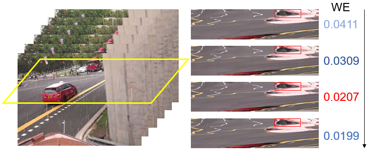
Fig. 6: Temporal slice comparison of rainy input, SGVD without ATC, full SGVD, and ground truth (top to bottom). ATC improves structural consistency across frames and reduces temporal artifacts, yielding a lower warping error (WE) .
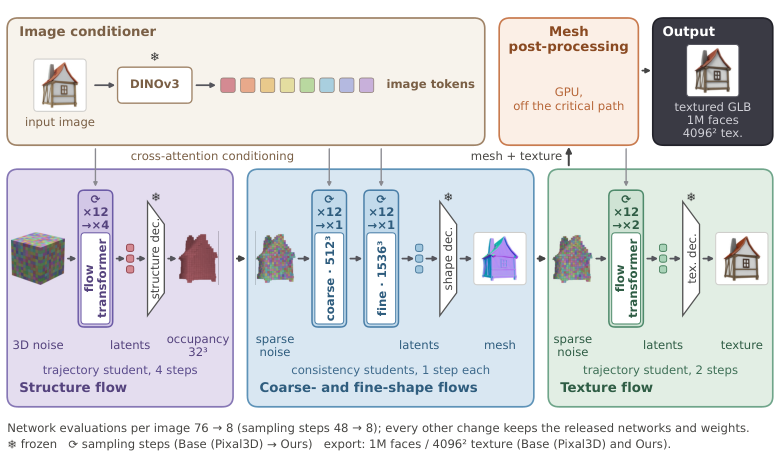
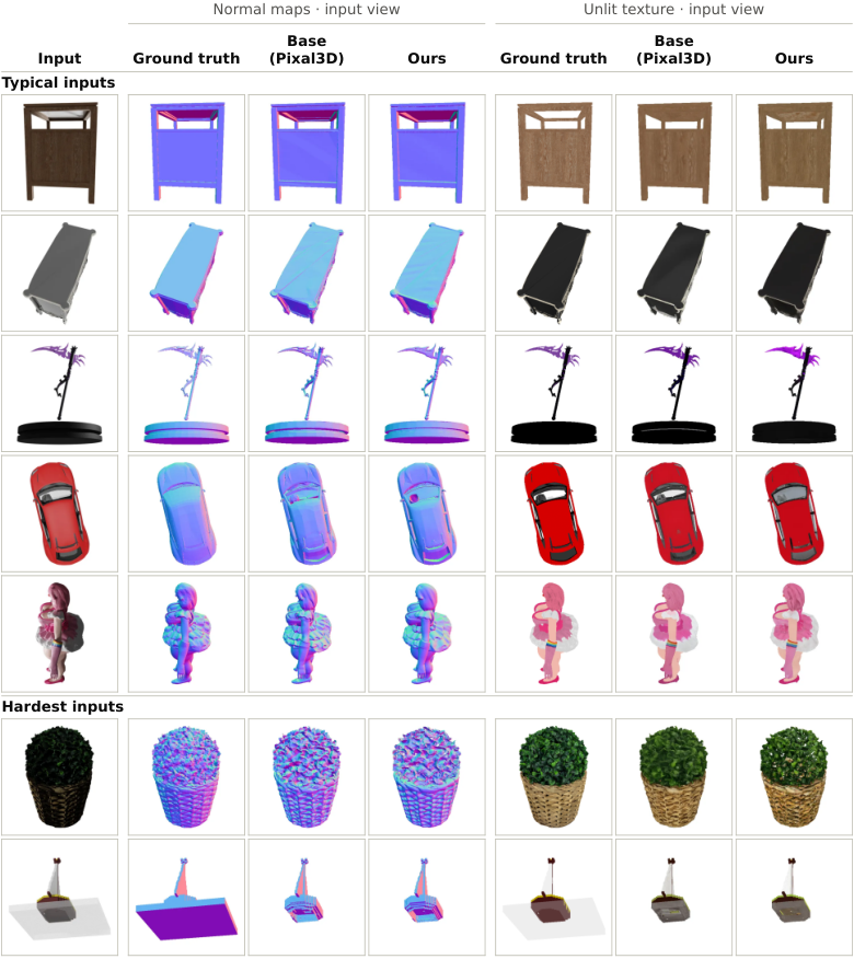
Figure 5 : Qualitative comparison. Seven inputs of the 40-object subset, rendered from the input camera: the input image, then the normal maps and the unlit base color of the ground truth, Base (Pixal3D) and Ours . Rows 1–5: typical inputs, in order of increasing angular error of Base (Pixal3D); rows 6–7: the two inputs with the largest error for Ours (selection: Section 4.4 ).
批判点评:33 倍是特定公开管线的全流程收益,并非所有图生 3D 网络自身快 33 倍;网格与蒸馏改动部分会改变输出,细纹理和几何对齐有代价。









评论 (0)