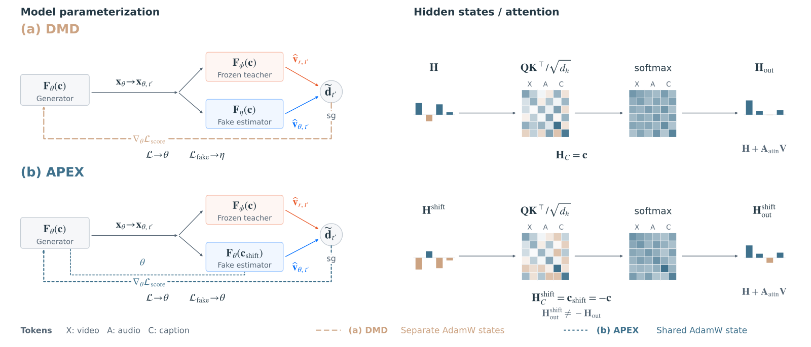
Figure 2 : DMD and APEX in Self-Replay Forcing. DMD uses independent fake parameters η \eta ; APEX shares generator and fake parameters θ \theta and, by default, AdamW states. Teacher parameters ϕ \phi are frozen. Left: θ \mathbf_{\theta} is the rollout/replay output, t ′ t^{\prime} the scoring time, ~ t ′ \widetilde{\mathbf{d}}_{t^{\prime}} the normalized correction, and sg \mathop{{\color[rgb]{1,0,0}\operatorname{sg}}}\nolimits stop-gradient. The correction contributes ∇ θ ℒ score \nabla_{\theta}\mathcal{L}_{\mathrm{score}} ; ℒ \mathcal{L} is the full generator objective. The fake-velocity subscript θ \theta identifies the generated distribution. Right: \mathbf{H} and out \mathbf{H}_{\mathrm{out}} denote input and output hidden states; C \mathbf{H}_{C} contains projected text tokens \mathbf{c} . Within each row, , , \mathbf{Q},\mathbf{K},\mathbf{V} are queries, keys, and values, and attn = softmax ( ⊤ / d h ) \mathbf{A}_{\mathrm{attn}}=\operatorname{softmax}(\mathbf{Q}\mathbf{K}^{\top}/\sqrt{d_{h}}) , with head dimension d h d_{h} . Superscript shift \mathrm{shift} marks states under shift = − \mathbf{c}_{\mathrm{shift}}=-\mathbf{c} . The single-head example uses fixed weights and omits the causal mask and other transformer operations; values are schematic.
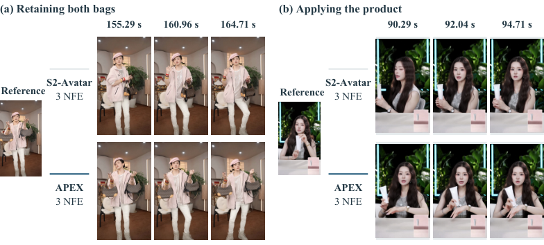
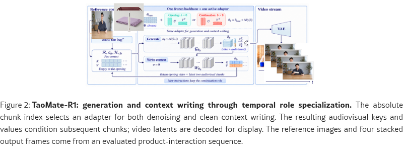
Figure 3 : Paired examples at 3 backbone NFE. (a) APEX retains both bags late in the sequence, while S2-Avatar shows one. (b) APEX brings the tube to the other hand for the applying instruction; S2-Avatar continues holding it at its side. Each pair uses the same reference and timestamps, with a common one-step 2 × 2\times Refiner.
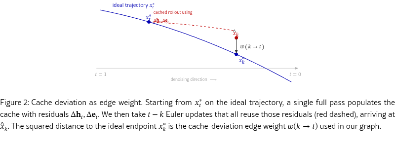
Figure 2: Cache deviation as edge weight. Starting from x t ∗ x_{t}^{*} on the ideal trajectory, a single full pass populates the cache with residuals Δ t , Δ t \Delta\mathbf{h}_{t},\Delta\mathbf{e}_{t} . We then take t − k t{-}k Euler updates that all reuse those residuals (red dashed), arriving at x ^ k \hat_{k} . The squared distance to the ideal endpoint x k ∗ x_{k}^{*} is the cache-deviation edge weight w ( k → t ) w(k\to t) used in our graph.
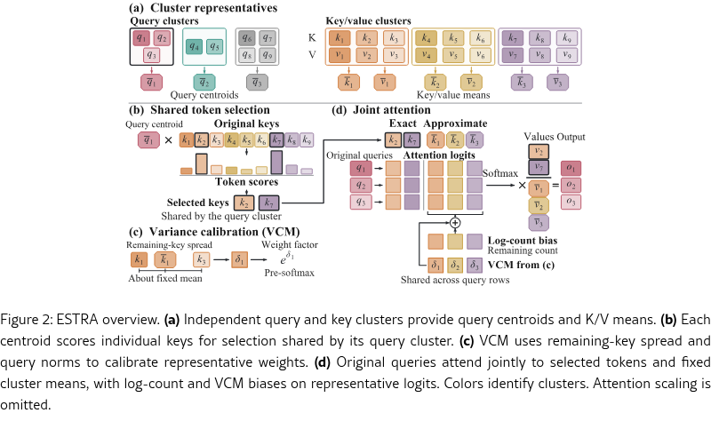
Figure 2: ESTRA overview. (a) Independent query and key clusters provide query centroids and K/V means. (b) Each centroid scores individual keys for selection shared by its query cluster. (c) VCM uses remaining-key spread and query norms to calibrate representative weights. (d) Original queries attend jointly to selected tokens and fixed cluster means, with log-count and VCM biases on representative logits. Colors identify clusters. Attention scaling is omitted.
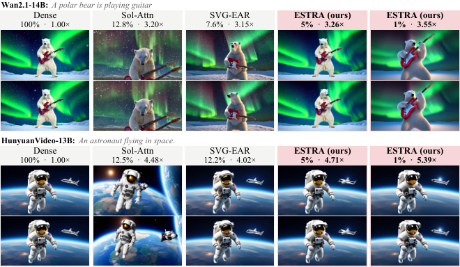
Figure 1: High-quality video generation at up to 99% attention sparsity. At 5% exact-interaction density, ESTRA more closely preserves the composition and appearance of the dense references than the baselines shown, while using higher sparsity and achieving greater end-to-end speedups. At 1%, the videos remain visually coherent, with particularly small changes in the HunyuanVideo example. Density denotes the fraction of video query–key interactions evaluated exactly; speedups are end to end on an NVIDIA H20. Additional examples are provided in Appendix D .
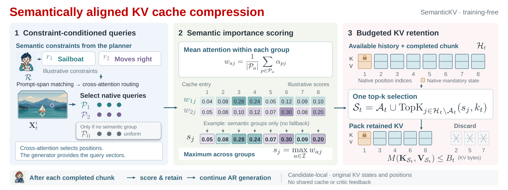
Figure 2: Overview of SemanticKV . Semantic constraints ℛ \mathcal{R} are matched to prompt tokens. Text cross-attention identifies related video positions, from which we collect the generator’s self-attention queries. Their attention to each KV entry is averaged within groups and maximized across groups. A single top- k k selection retains high-scoring entries within the byte budget, together with states required by the backbone. Retained keys, values, and positions remain unchanged.
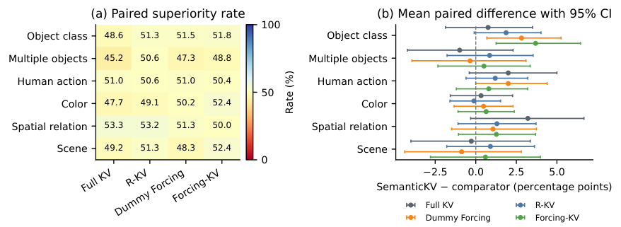
Figure 4: Paired semantic fidelity on matched prompt–seed tuples. (a) Tie-aware superiority rates. (b) Mean paired differences with prompt-clustered bootstrap 95% confidence intervals. Positive differences favor SemanticKV ; Full KV is the uncompressed reference.
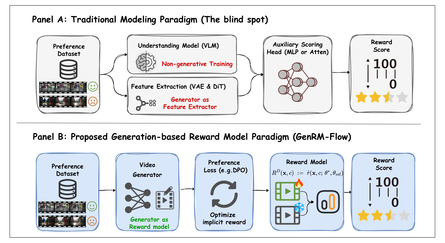
Figure 2: The pipeline of GenRM-Flow . (Panel A) Traditional paradigms rely on representational capacity , utilizing a frozen backbone (e.g., a VLM or base generator) as a feature extractor coupled with an auxiliary discriminative head. (Panel B) The proposed framework sources the reward directly from generative capacity . Following preference optimization, the implicit reward R D ( , c ) R^{D}(\mathbf,c) is algebraically extracted from the velocity-prediction errors. The scalar score is computed natively by contrasting the active policy (flame, θ ⋆ \theta^{\star} ) against a frozen reference (snowflake, θ ref \theta_{\mathrm{ref}} ), requiring no architectural modifications or auxiliary heads.
Figure 4: Qualitative comparison between PAVRM and GenRM-Flow as the per-step reward signal in FlowAWR with a 1.3B backbone. Both runs use FlowAWR with the same configuration, differing only in the reward signal. Red boxes mark localized structural deformations, spatial inconsistencies, and temporal artifacts produced by PAVRM. Across scenes, our reward yields visibly fewer geometric defects and better spatial and temporal continuity.
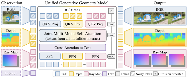
Figure 2: Generative-predictive transformer. We model RGB, depth, and camera pose as spatially aligned tokens, with camera pose represented as dense ray maps. Partial observations are zero-noise context tokens, while missing modalities are noisy tokens to be denoised. A unified transformer processes all tokens with modality-specific projections and feed-forward layers together with shared multimodal self-attention, enabling information exchange across modalities. The decoded RGB, depth, and ray maps form a complete 4D scene representation for cross-modal generation, geometric prediction, and inference-time consistency search.
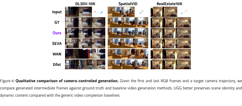
实验效果:RealEstate10K 双端点帧加目标相机轨迹的视频补全中,UGG 的 峰值信噪比 PSNR 为 25.73 dB、感知距离 LPIPS 为 0.061,对照 SEVA 为 25.25 dB、0.081;PSNR 越高、LPIPS 越低通常表示与真值更接近。但 DL3DV 同设定中,UGG 的 PSNR 16.61 dB 低于 SEVA 的 17.61 dB。
Figure 4: Qualitative comparison of camera-controlled generation. Given the first and last RGB frames and a target camera trajectory, we compare generated intermediate frames against ground truth and baseline video generation methods. UGG better preserves scene identity and dynamic content compared with the generic video completion baselines.
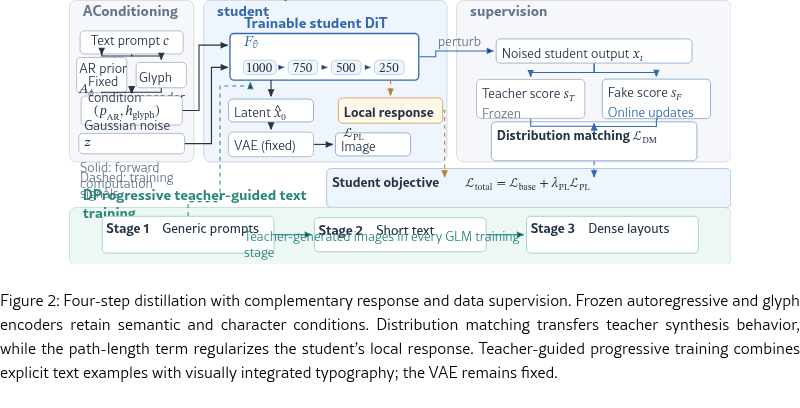
Figure 2: Four-step distillation with complementary response and data supervision. Frozen autoregressive and glyph encoders retain semantic and character conditions. Distribution matching transfers teacher synthesis behavior, while the path-length term regularizes the student’s local response. Teacher-guided progressive training combines explicit text examples with visually integrated typography; the VAE remains fixed.
Figure 6: Qualitative comparison of four-step GLM-Image students. Within each three-column group, outputs are ordered as the student without text training, TDM, and our complete framework. Cases cover (a) an English poster, (b) a Chinese poster, (c) a bilingual sign, (d) product packaging, (e) multiline text, (f) a bilingual display, (g) object counting, and (h) spatial relations. The examples illustrate differences in literal text preservation, object counts, and spatial arrangement while retaining coherent scene appearance.
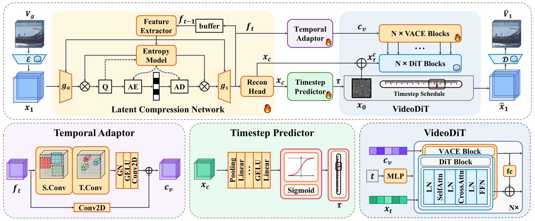
Figure 3 : The overall architecture of ADE-GVC consists of a latent compression network (LCN), temporal adaptor (TA), timestep predictor (TP), and video diffusion model. The input video g \bm{V}_{g} is encoded into the clean latent 1 \bm_{1} , which is compressed by the LCN into c \bm_{c} and a compression-aware feature t \bm{f}_{t} . The TP predicts the denoising entry τ \tau from c \bm_{c} , while the TA converts t \bm{f}_{t} into the visual context v \bm{c}_{v} . Conditioned on v \bm{c}_{v} , the VideoDiT denoises τ c \bm^{c}_{\tau} , into ^ 1 \hat{\bm}_{1} , which is decoded to reconstruct ^ 1 \hat{\bm{V}}_{1} .
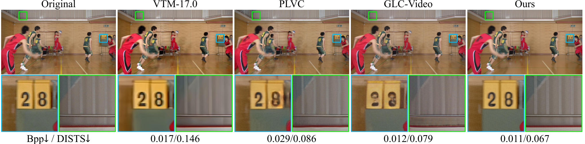
Figure 7 : Qualitative comparisons on a single frame in terms of representative VVC, PLVC, GLC-Video and our ADE-GVC methods. We also report the Bpp/DISTS metrics to quantify compression efficiency.
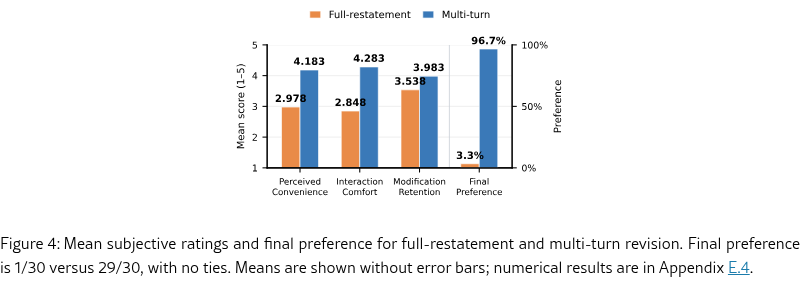
Figure 4: Mean subjective ratings and final preference for full-restatement and multi-turn revision. Final preference is 1/30 versus 29/30, with no ties. Means are shown without error bars; numerical results are in Appendix E.4 .
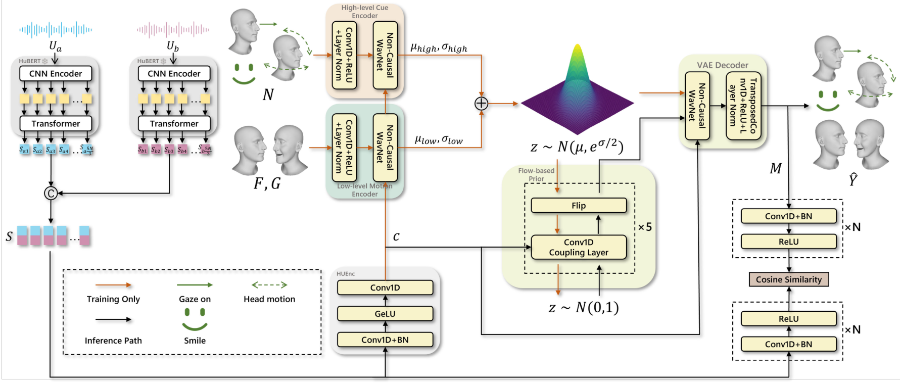
Fig. 2: Overview of the proposed DiaHeads. The audio streams of both interlocutors are encoded by two frozen HuBERT backbones and fused into a conditioning vector c c by a transformer. A dual-branch variational encoder processes the continuous parameters ( F , G ) (F,G) and the discrete cues N N in separate branches, each conditioned on c c through FiLM modulation, and the two branches are combined through a product-of-experts posterior z ∼ ( μ , e σ / 2 ) z\sim\mathcal{N}(\mu,e^{\sigma/2}) , shown as the “Low-level Motion Encoder” and “High-level Cue Encoder”. A flow-based prior built from five residual coupling blocks, each consisting of a flip operation and a Conv1D coupling layer, replaces the standard Gaussian prior, and a shared VAE decoder, conditioned on c c through FiLM, jointly reconstructs the head parameters Y ^ \hat{Y} and the discrete cues of both interlocutors. The units at the bottom right detail the two SyncNet encoders, which are built from 1D convolution, batch normalization, and ReLU.
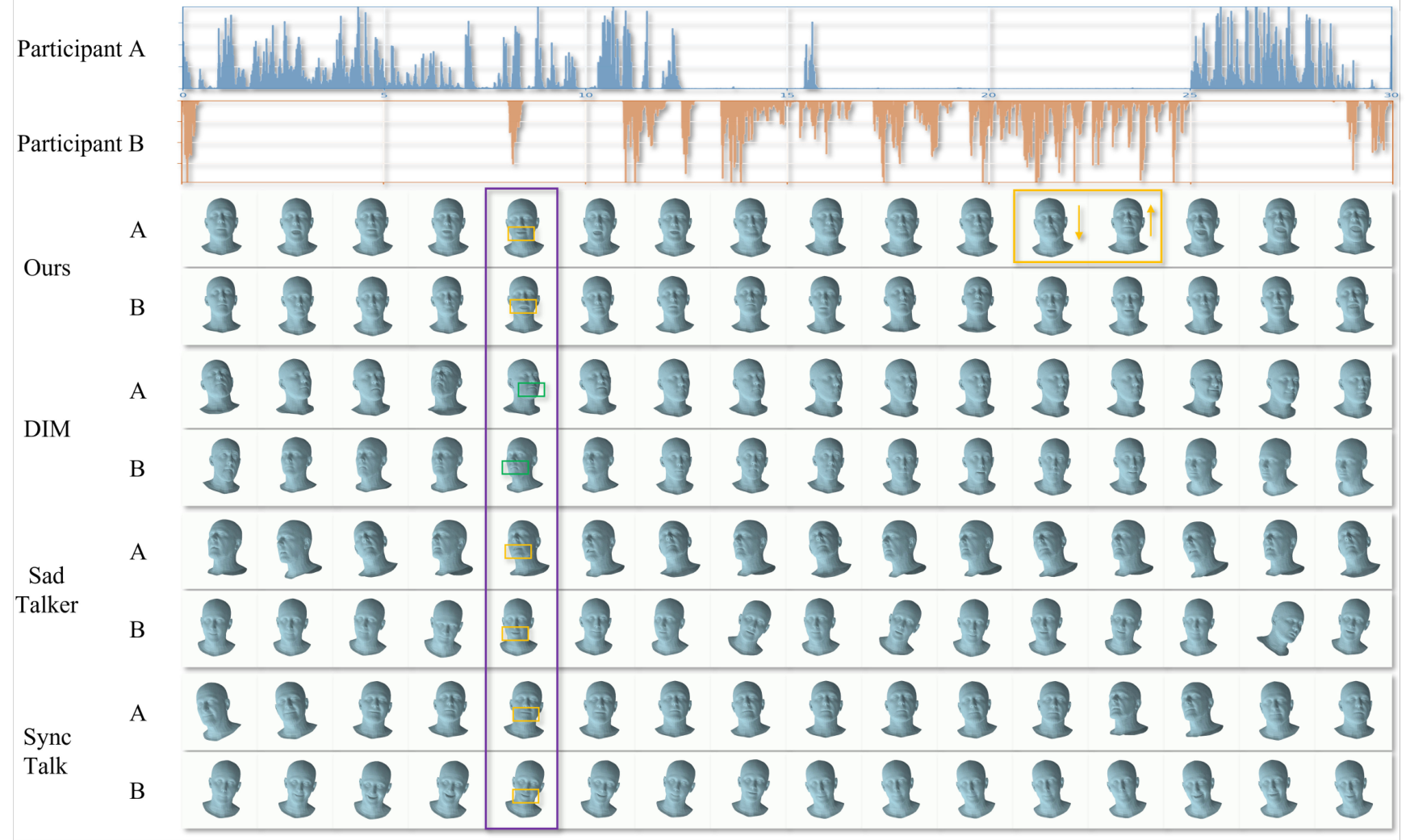
Fig. 5: Qualitative comparison of generated 3D head animations over a 30 s dialogue clip. Participant A is shown in blue and participant B in orange. Each method occupies two rows labeled A and B, sampled every 2.5 s. Our method produces appropriate mouth movements during overlapping speech at 8 s, marked by the purple box, and responsive nodding with mutual gaze at 20–23 s, marked by the yellow box, while the baselines show incorrect lip-sync and lack interactive behaviors.
批判点评:论文展示的是 3D 头像动画参数,不是直接输出真人视频;双人数据和四种 cue 限制了外推范围。交互协调改善与单人几何误差存在取舍;原文仅称准备投稿 IEEE Transactions on Multimedia,未写成已接收。









评论 (0)