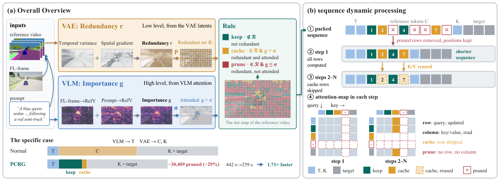
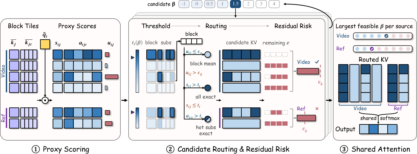
Figure 2 : Overview of PCRG. (a) Before step 1, the redundancy r r of the VAE latents selects the redundant set ℛ \mathcal{R} , the most redundant fraction ρ \rho of each block. The importance g g from the VLM marks the cells with g > σ g>\sigma as attended. (b) Pruned rows leave the packed sequence, and the remaining tokens keep their RoPE (①). Step 1 computes every remaining row (②). Steps 2– N N skip the cached rows and reuse their keys and values from step 1 (③). In the attention maps (④), from step 2 on, a cached token keeps its key column but loses its query row, and a pruned token has neither.
Figure 3 : Qualitative comparison on a V2V-Bench request. GT is the unpruned output, and the number in parentheses is the LPIPS to it. +TeaCache and +Spark combine PCRG with TeaCache and Spark.
Figure 1 : Motion-aware reward model. The pixel stream encodes source and edited videos, while a dynamics stream computes tanh-normalized RGB differences of the edited video. Their features are fused at block 4 of the Qwen3-VL-32B backbone and adapted with LoRA. Training combines pairwise preferences over original edits and motion-suppressed or fabricated-motion negatives with a distillation anchor to the base preference reward.
Figure S1 : Motion ladders for three VE-Bench edits. Columns show six uniformly sampled frames. Hold-2 and hold-4 repeat every second or fourth frame, respectively; frozen repeats the first frame. Variants retain the clip length but use subsets of the original frames.
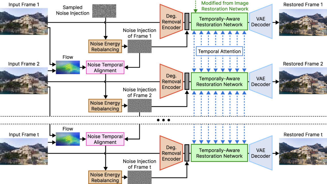
Figure 7 : Overview of the proposed video restoration framework. Noise energy rebalancing, motion-aligned noise propagation, and temporal attention are jointly applied in a sequence-to-sequence manner to achieve temporally consistent restoration.
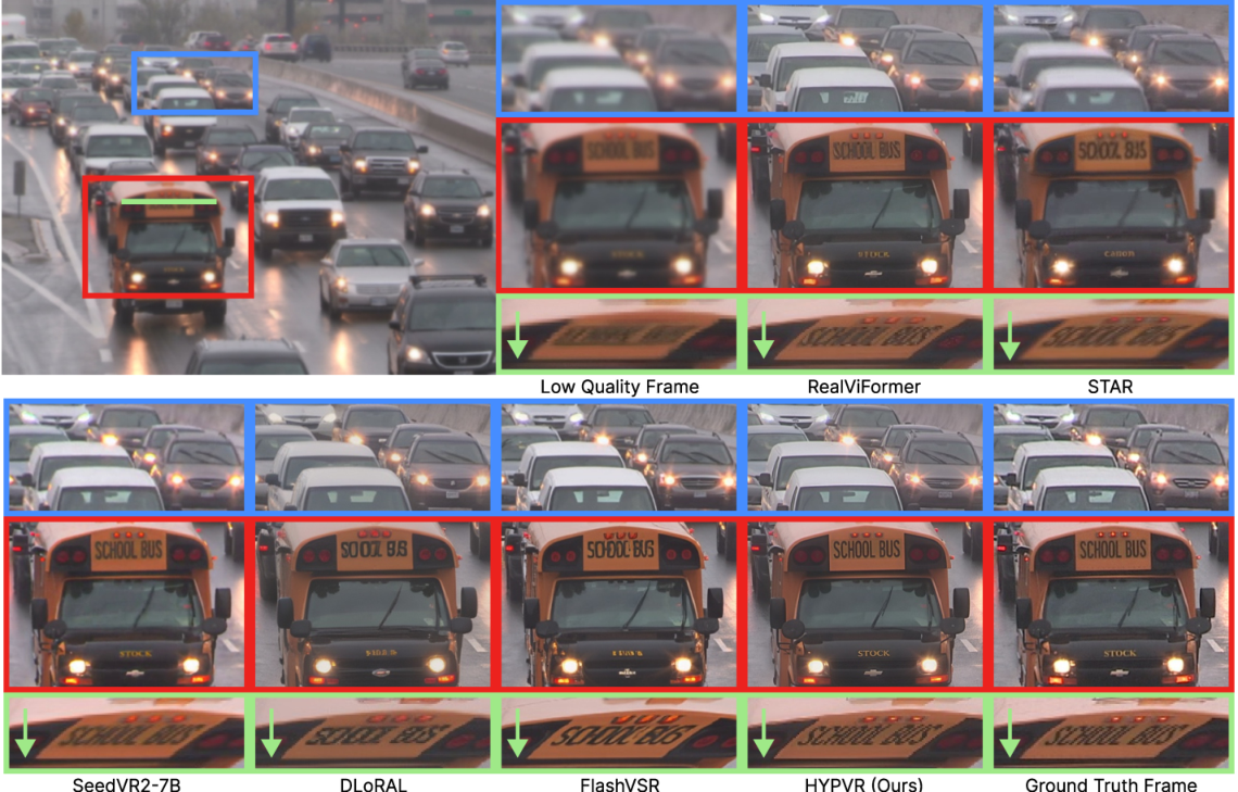
Figure 8 : Qualitative and temporal profile comparison. HYPI2VR restores semantically meaningful details while preserving high temporal coherence and visual stability across frames.
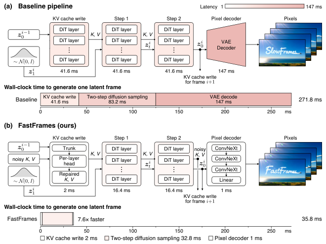
Figure 2 : Inference pipeline and latency profiling for one autoregressive generation. State-of-the-art few-step autoregressive video diffusion models generate each new frame by first updating the KV cache using the previous frame’s denoised latent ( 0 i − 1 {\bm{z}}^{i-1}_{0} ) through a DiT evaluation, then performing multiple denoising steps followed by VAE decoding. The color gradient of the model components denotes speed: from white (fastest operations) to red (slowest). (a) The fastest baseline, Causal Forcing++ ( Zhao et al., 2026a ) , takes 271 ms to generate a frame at 480p but only 30% of wall time is spent on diffusion sampling. (b) FastFrames reduces latency nearly 8× by replacing the non-denoising “accessories” with lightweight alternatives and performing systems-level optimizations to speed up each DiT evaluation.
Figure 5 : Interactive generation and latency results. Left: example of interaction with LingBot’s official implementation vs. with FastFrames optimizations. Given a single keypress, FastFrames is 16× faster to respond. Right: generation latency of officially released implementations and our optimized implementations. We measure steady-state latency on NVIDIA B200 GPUs at 832×480 resolution with a full KV cache and include distributed optimizations such as Ulysses where officially supported. Times include diffusion sampling (four steps for LingBot and three for RealWonder), action conditioning, KV-cache updates, and pixel decoding. Our optimizations provide speedups of 3× to 22×. See the project website for the video demonstration.
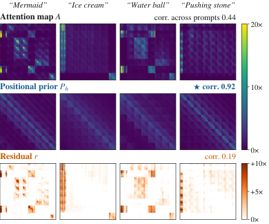
Figure 4 : Attention decomposes into an input-stable positional prior and an input-dependent content residual. Each column corresponds to a different prompt. The bottom row shows the residual attention that content adds on top of the positional prior.
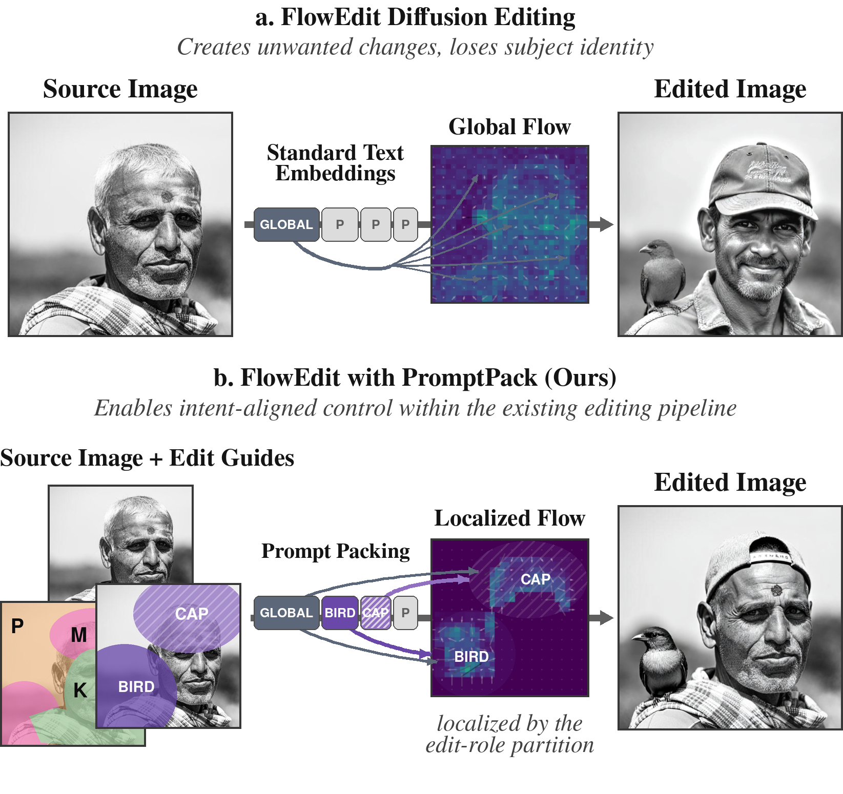
Figure 1 : PromptPack adds explicit spatial and semantic control to an existing editing pipeline. (a) FlowEdit: global text conditioning is applied throughout the image, producing unwanted changes and losing subject identity. (b) PromptPack: the user marks where a “bird” and a “cap” should appear and identifies the man’s face and scarf as content to preserve. PromptPack translates these annotations into the edit-role partition and regional-prompt assignment shown at left, packs global and regional text embeddings into the conditioning sequence, and routes them to spatially localized flow supports. This enables intent-aligned control.
Figure 2 : Qualitative comparisons across the three evaluated integrations. Rows 1 and 3 show the source images and user-provided text required by each baseline editor. FlowEdit FLUX and FlowEdit SD3 use source and target descriptions, whereas FLUX Kontext uses a single edit instruction. Baseline outputs may alter unrelated content or incompletely realize requested concepts (row 4). PromptPack retains the same text conditioning and adds the Edit Guides in row 2, producing outputs that better follow the requested spatial intent while preserving unrelated content (row 5). For these PIE-Bench++ examples, we draw one concept-placement box per requested addition. Each box is an assignment mask; their union initializes Modify , a dilation collar defines Permit , and the remainder defines Keep . Solid and striped swatches link the regional prompts in row 3 to their assignment masks. Architecture-specific mappings are detailed in the supplement.
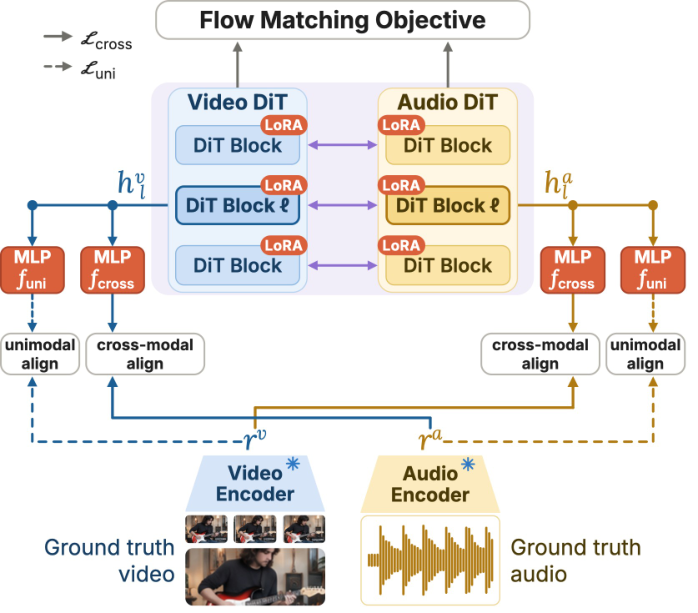
Figure 5 : Overview of JointREPA. JointREPA aligns each modality’s features with pretrained encoder representations from both its own modality and the other modality.
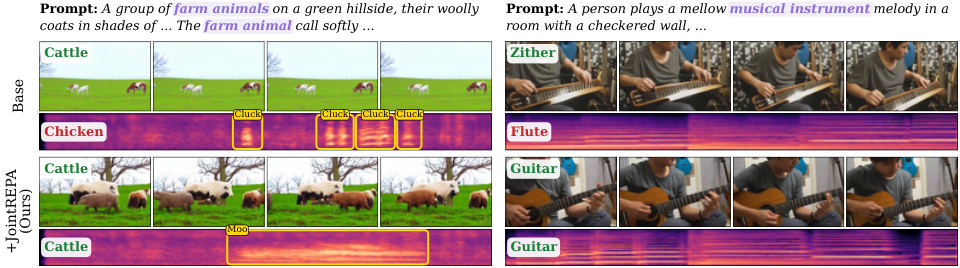
Figure 6 : Qualitative results on UNSAIDBench. Generated video frames and audio spectrograms from the base model (top) and its JointREPA variant (bottom). Given an underspecified shared factor per prompt, the base model realizes different semantic identities in audio and video, whereas JointREPA converges on the same identity.
批判点评:一致性提升带来质量取舍:UNSAIDBench 上 LTX-2.3 的 VQ 和 AQ 均下降。自动指标仍受编码器与提示集影响;JointREPA 另需后训练与双模态编码器,不能把内在协同性提升等同于所有感官质量改善。
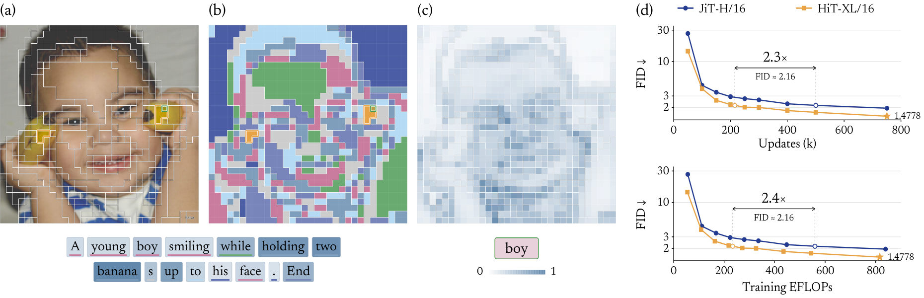
Figure 1 : HiT learns image–text associations without region annotations and converges faster. (a) On a clean input ( t = 1 t=1 ), HiT groups patches with similar representations. (b) The corresponding group map. Spatially disconnected patches from both bananas share the yellow group. Darker blue caption words indicate stronger soft routing connections from the banana patch outlined in green. (c) For the selected word “boy”, the image heatmap shows its group’s soft pooling weights, emphasizing the boy’s face and upper body. (d) FID-50k on a log scale for HiT-XL/16 and JiT-H/16 on ImageNet-256, using guidance scales 2.6 2.6 and 2.4 2.4 , respectively, plotted against optimizer updates (top) and estimated cumulative training compute (bottom). At FID ≈ 2.16 \approx 2.16 , HiT uses 2.4 × 2.4\times less training compute and 2.3 × 2.3\times fewer updates.
Figure 7 : Image groups at stage 2. All examples use clean inputs at t = 1 t=1 . Rows show an airport scene, a stop sign, orange peels, and a baseball scene. The left column shows the full group map. Each of the three remaining panels highlights one selected group in yellow. White lines show all hard group boundaries. Colors distinguish touching groups and can repeat in distant groups.
批判点评:训练 FLOPs、前向 FLOPs 与实际墙钟时间是不同口径;分组和展开也有计算成本,机构署名及完整实验配置仍需从原文 PDF 核定。
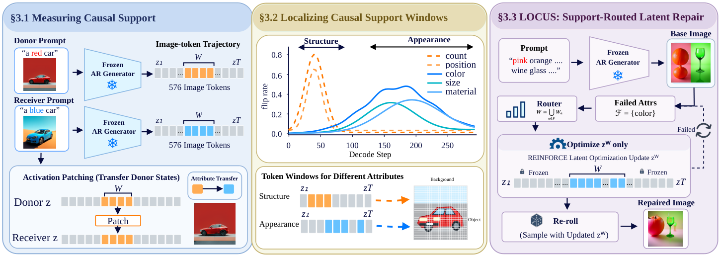
9. LOCUS:按失败属性定位图像 token
LOCUS: Causal Support Windows for Attribute Control in Autoregressive Image Generation | 独立研究者 | arXiv:2611.22867
Figure 2 : Overview of LOCUS. § 3.1 measures causal support C a ( W ) C_{a}(W) by cross-prompt activation patching: donor hidden states replace the receiver’s over a window W W , and the flip rate is the support. § 3.2 locates each attribute’s support window on the image-token trajectory: count and position peak early and narrowly, while color, size, and material peak in the mid band over the object body. § 3.3 diagnoses a failed generation, routes optimization to the union of the failed attributes’ windows under a fixed token budget, and updates only those latents with REINFORCE while the generator stays frozen.
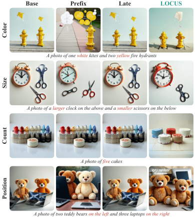
Figure 8 : Qualitative comparison under a matched budget. All images are real generations; the target cue is highlighted in red under each row. Rows cover appearance (color, size) and structure (count, position) failures, and columns compare the base image with the prefix, late, and LOCUS windows.
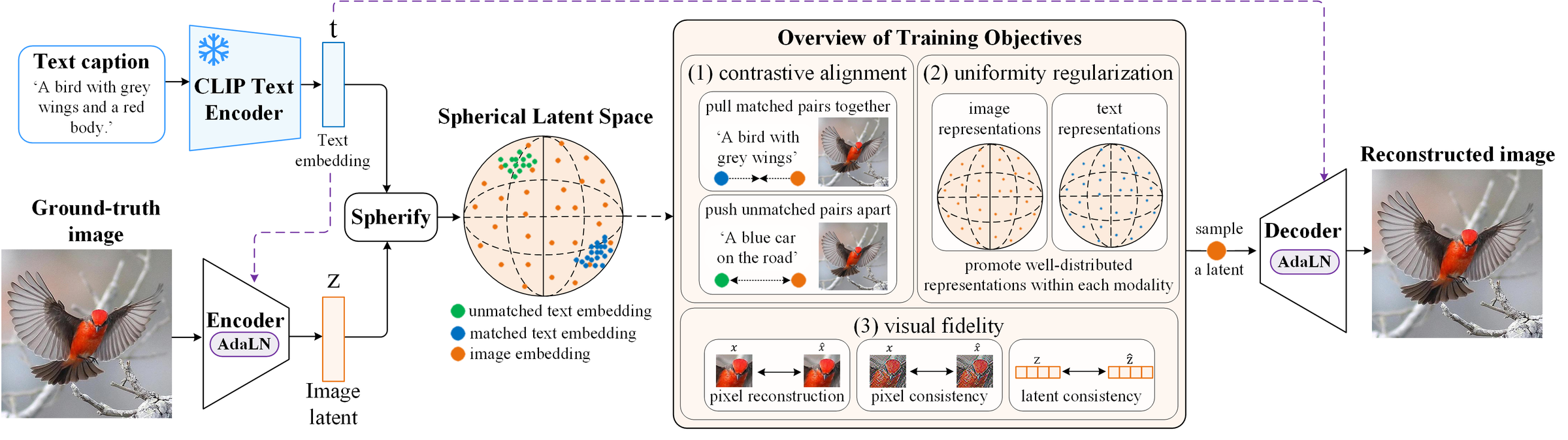
Figure 2 : TextSphere Framework Overview. It consists of a frozen pretrained CLIP text encoder, an image encoder, and an image decoder. During training, the image encoder maps ground-truth images onto a spherical latent space via RMS normalization (Spherify), as defined in Eq. ( 1 ), while the CLIP text encoder extracts semantic embeddings \mathbf{t} from the corresponding captions. The training objectives jointly optimize (1) contrastive alignment, (2) uniformity regularization, and (3) visual fidelity, with the decoder sampling random latent representations from the hypersphere to generate images.











评论 (0)